Adjust the luminance for a palette of colors
Description
The adjust_luminance() function can brighten or darken a palette of colors
by an arbitrary number of steps, which is defined by a real number between
-2.0 and 2.0. The transformation of a palette by a fixed step in this
function will tend to apply greater darkening or lightening for those colors
in the midrange compared to any very dark or very light colors in the input
palette.
Usage
adjust_luminance(colors, steps)adjust_luminance(colors, steps)
Arguments
colors |
Color vector
This is the vector of colors that will undergo an adjustment in luminance.
Each color value provided must either be a color name (in the set of colors
provided by |
steps |
Adjustment level
A positive or negative factor by which the luminance of colors in the
|
Details
This function can be useful when combined with the data_color() function's
palette argument, which can use a vector of colors or any of the col_*
functions from the scales package (all of which have a palette
argument).
Value
A vector of color values.
Examples
Get a palette of 8 pastel colors from the RColorBrewer package.
pal <- RColorBrewer::brewer.pal(8, "Pastel2")
Create lighter and darker variants of the base palette (one step lower, one step higher).
pal_darker  <- pal |> adjust_luminance(-1.0)
pal_lighter <- pal |> adjust_luminance(+1.0)
Create a tibble and make a gt table from it. Color each column in order
of increasingly darker palettes (with data_color()).
dplyr::tibble(a = 1:8, b = 1:8, c = 1:8) |>
  gt() |>
  data_color(
    columns = a,
    colors = scales::col_numeric(
      palette = pal_lighter,
      domain = c(1, 8)
    )
  ) |>
  data_color(
    columns = b,
    colors = scales::col_numeric(
      palette = pal,
      domain = c(1, 8)
    )
  ) |>
  data_color(
    columns = c,
    colors = scales::col_numeric(
      palette = pal_darker,
      domain = c(1, 8)
    )
  )

Function ID
8-9
Function Introduced
v0.2.0.5 (March 31, 2020)
See Also
Other helper functions:
cell_borders(),
cell_fill(),
cell_text(),
currency(),
default_fonts(),
escape_latex(),
from_column(),
google_font(),
gt_latex_dependencies(),
html(),
latex(),
md(),
nanoplot_options(),
pct(),
px(),
random_id(),
row_group(),
stub(),
system_fonts(),
unit_conversion()
Transform a gt table to a gtable object
Description
as_gtable() performs the transformation of a gt_tbl object to a
gtable object.
Usage
as_gtable(data, plot = FALSE, text_grob = grid::textGrob)as_gtable(data, plot = FALSE, text_grob = grid::textGrob)
Arguments
data |
The gt table data object
This is the gt table object that is commonly created through use of the
|
plot |
Render through the graphics device?
The |
text_grob |
Function for drawing text
A |
Value
A gtable object.
Function ID
13-6
Function Introduced
v0.11.0 (July 9, 2024)
See Also
Other table export functions:
as_latex(),
as_raw_html(),
as_rtf(),
as_word(),
extract_body(),
extract_cells(),
extract_summary(),
gtsave()
Output a gt object as LaTeX
Description
Get the LaTeX content from a gt_tbl object as a knit_asis object. This
object contains the LaTeX code and attributes that serve as LaTeX
dependencies (i.e., the LaTeX packages required for the table). Using
as.character() on the created object will result in a single-element vector
containing the LaTeX code.
Usage
as_latex(data)as_latex(data)
Arguments
data |
The gt table data object
This is the gt table object that is commonly created through use of the
|
Details
LaTeX packages required to generate tables are: booktabs, caption, longtable, colortbl, array, anyfontsize, multirow.
In the event packages are not automatically added during the render phase of the document, please create and include a style file to load them.
Inside the document's YAML metadata, please include:
output:
  pdf_document: # Change to appropriate LaTeX template
    includes:
      in_header: 'gt_packages.sty'
The gt_packages.sty file would then contain the listed dependencies above:
\usepackage{booktabs, caption, longtable, colortbl, array}
Examples
Use a subset of the gtcars dataset to create a gt table. Add a header
with tab_header() and then export the table as LaTeX code using the
as_latex() function.
tab_latex <-
  gtcars |>
  dplyr::select(mfr, model, msrp) |>
  dplyr::slice(1:5) |>
  gt() |>
  tab_header(
    title = md("Data listing from **gtcars**"),
    subtitle = md("`gtcars` is an R dataset")
  ) |>
  as_latex()
What's returned is a knit_asis object, which makes it easy to include in R
Markdown documents that are knit to PDF. We can use as.character() to get
just the LaTeX code as a single-element vector.
Function ID
13-3
Function Introduced
v0.2.0.5 (March 31, 2020)
See Also
Other table export functions:
as_gtable(),
as_raw_html(),
as_rtf(),
as_word(),
extract_body(),
extract_cells(),
extract_summary(),
gtsave()
Get the HTML content of a gt table
Description
Get the HTML content from a gt_tbl object as a single-element character
vector. By default, the generated HTML will have inlined styles, where CSS
styles (that were previously contained in CSS rule sets external to the
<table> element) are included as style attributes in the HTML table's
tags. This option is preferable when using the output HTML table in an
emailing context.
Usage
as_raw_html(data, inline_css = TRUE)as_raw_html(data, inline_css = TRUE)
Arguments
data |
The gt table data object
This is the gt table object that is commonly created through use of the
|
inline_css |
Use inline CSS
An option to supply styles to table elements as inlined CSS styles. This is
useful when including the table HTML as part of an HTML email message body,
since inlined styles are largely supported in email clients over using CSS
in a |
Examples
Use a subset of the gtcars dataset to create a gt table. Add a header
with tab_header() and then export the table as HTML code with inlined CSS
styles using as_raw_html().
tab_html <-
  gtcars |>
  dplyr::select(mfr, model, msrp) |>
  dplyr::slice_head(n = 5) |>
  gt() |>
  tab_header(
    title = md("Data listing from **gtcars**"),
    subtitle = md("`gtcars` is an R dataset")
  ) |>
  as_raw_html()
What's returned is a single-element vector containing the HTML for the table.
It has only the <table>...</table> part so it's not a complete HTML
document but rather an HTML fragment.
Function ID
13-2
Function Introduced
v0.2.0.5 (March 31, 2020)
See Also
Other table export functions:
as_gtable(),
as_latex(),
as_rtf(),
as_word(),
extract_body(),
extract_cells(),
extract_summary(),
gtsave()
Output a gt object as RTF
Description
Get the RTF content from a gt_tbl object as as a single-element character
vector. This object can be used with writeLines() to generate a valid .rtf
file that can be opened by RTF readers.
Usage
as_rtf( data, incl_open = TRUE, incl_header = TRUE, incl_page_info = TRUE, incl_body = TRUE, incl_close = TRUE )as_rtf( data, incl_open = TRUE, incl_header = TRUE, incl_page_info = TRUE, incl_body = TRUE, incl_close = TRUE )
Arguments
data |
The gt table data object
This is the gt table object that is commonly created through use of the
|
incl_open, incl_close
|
Include opening/closing braces
Options that govern whether the opening or closing |
incl_header |
Include RTF header
Should the RTF header be included in the output? By default, this is
|
incl_page_info |
Include RTF page information
Should the RTF output include directives for the document pages? This is
|
incl_body |
Include RTF body
An option to include the body of RTF document. By default, this is |
Examples
Use a subset of the gtcars dataset to create a gt table. Add a header
with tab_header() and then export the table as RTF code using the
as_rtf() function.
tab_rtf <-
  gtcars |>
  dplyr::select(mfr, model) |>
  dplyr::slice(1:2) |>
  gt() |>
  tab_header(
    title = md("Data listing from **gtcars**"),
    subtitle = md("`gtcars` is an R dataset")
  ) |>
  as_rtf()
Function ID
13-4
Function Introduced
v0.2.0.5 (March 31, 2020)
See Also
Other table export functions:
as_gtable(),
as_latex(),
as_raw_html(),
as_word(),
extract_body(),
extract_cells(),
extract_summary(),
gtsave()
Output a gt object as Word
Description
Get the Open Office XML table tag content from a gt_tbl object as a
single-element character vector.
Usage
as_word( data, align = "center", caption_location = c("top", "bottom", "embed"), caption_align = "left", split = FALSE, keep_with_next = TRUE, autonum = TRUE )as_word( data, align = "center", caption_location = c("top", "bottom", "embed"), caption_align = "left", split = FALSE, keep_with_next = TRUE, autonum = TRUE )
Arguments
data |
The gt table data object
This is the gt table object that is commonly created through use of the
|
align |
Table alignment
An option for table alignment. Can either be |
caption_location |
Caption location
Determines where the caption should be positioned. This can either be
|
caption_align |
Caption alignment Determines the alignment of the caption. This is
either |
split |
Allow splitting of a table row across pages
A logical value that indicates whether to activate the Word option
|
keep_with_next |
Keeping rows together
A logical value that indicates whether a table should use Word option
|
autonum |
Automatic Table Numbering
A logical value that indicates whether a table should use Words built-in
auto table numbering option in the caption.
|
Examples
Use a subset of the gtcars dataset to create a gt table. Add a header
with tab_header() and then export the table as OOXML code for Word using
as_word()
tab_rtf <-
  gtcars |>
  dplyr::select(mfr, model) |>
  dplyr::slice(1:2) |>
  gt() |>
  tab_header(
    title = md("Data listing from **gtcars**"),
    subtitle = md("`gtcars` is an R dataset")
  ) |>
  as_word()
Function ID
13-5
Function Introduced
v0.7.0 (August 25, 2022)
See Also
Other table export functions:
as_gtable(),
as_latex(),
as_raw_html(),
as_rtf(),
extract_body(),
extract_cells(),
extract_summary(),
gtsave()
Helper for defining custom borders for table cells
Description
cell_borders() is to be used with tab_style(), which itself allows for
the setting of custom styles to one or more cells. Specifically, the call to
cell_borders() should be bound to the styles argument of tab_style().
The sides argument is where we define which borders should be modified
(e.g., "left", "right", etc.). With that selection, the color, style,
and weight of the selected borders can then be modified.
Usage
cell_borders(sides = "all", color = "#000000", style = "solid", weight = px(1))cell_borders(sides = "all", color = "#000000", style = "solid", weight = px(1))
Arguments
sides |
Border sides
The border sides to be modified. Options include |
color |
Border color
The border |
style |
Border line style
The border |
weight |
Border weight
The default value for |
Value
A list object of class cell_styles.
Examples
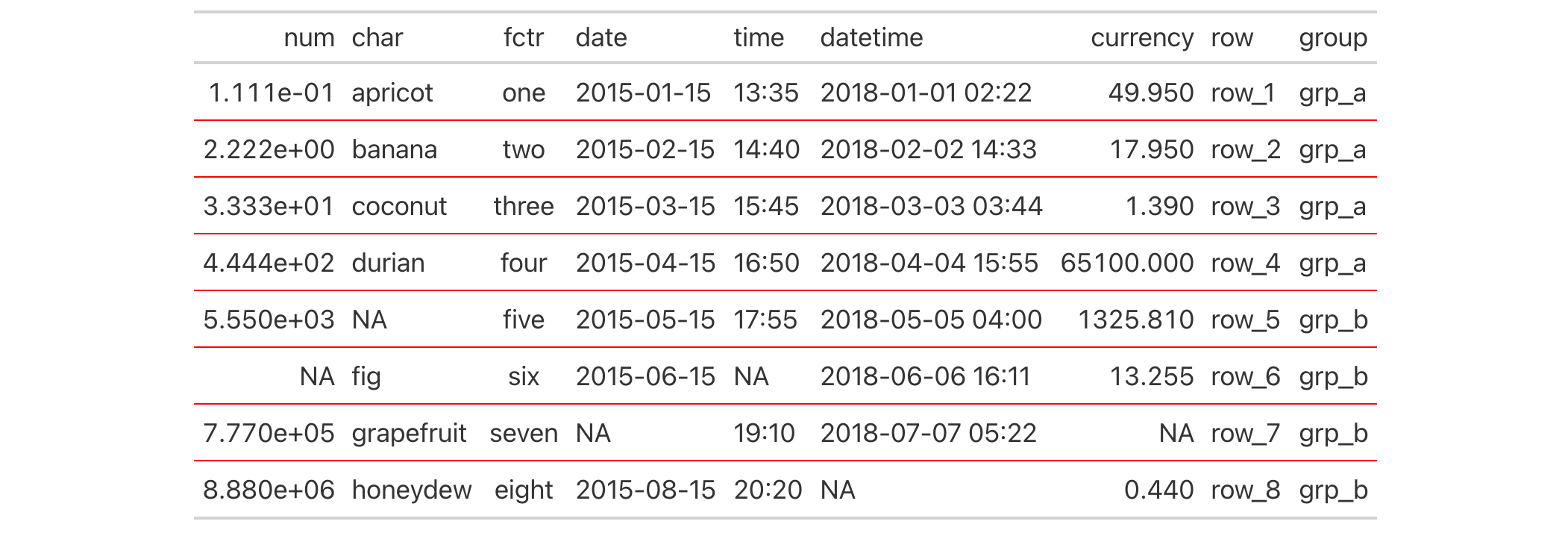
We can add horizontal border lines for all table body rows in a gt table
based on the exibble dataset. For this, we need to use tab_style()
(targeting all cells in the table body with cells_body()) in conjunction
with cell_borders() in the style argument. Both top and bottom borders
will be added as "solid" and "red" lines with a line width of 1.5 px.
exibble |>
  gt() |>
  tab_style(
    style = cell_borders(
      sides = c("top", "bottom"),
      color = "red",
      weight = px(1.5),
      style = "solid"
    ),
    locations = cells_body()
  )
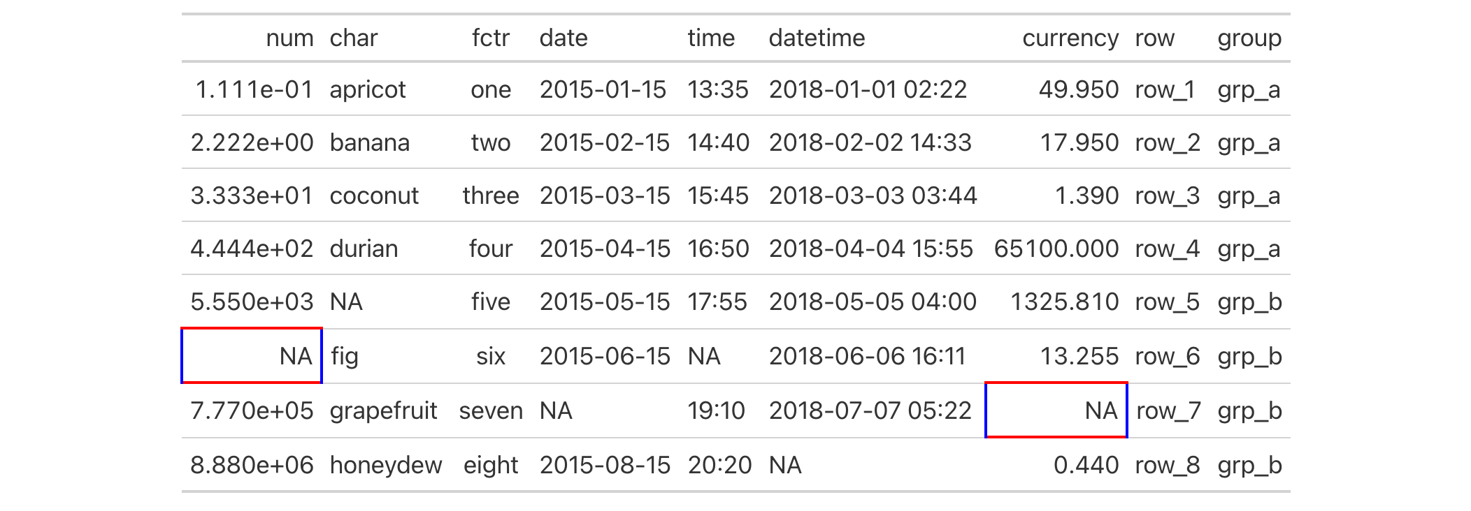
It's possible to incorporate different horizontal and vertical ("left" and
"right") borders at several different locations. This uses multiple
cell_borders() and cells_body() calls within their own respective lists.
exibble |>
  gt() |>
  tab_style(
    style = list(
      cell_borders(
        sides = c("top", "bottom"),
        color = "#FF0000",
        weight = px(2)
      ),
      cell_borders(
        sides = c("left", "right"),
        color = "#0000FF",
        weight = px(2)
      )
    ),
    locations = list(
      cells_body(
        columns = num,
        rows = is.na(num)
      ),
      cells_body(
        columns = currency,
        rows = is.na(currency)
      )
    )
  )
Function ID
8-27
Function Introduced
v0.2.0.5 (March 31, 2020)
See Also
Other helper functions:
adjust_luminance(),
cell_fill(),
cell_text(),
currency(),
default_fonts(),
escape_latex(),
from_column(),
google_font(),
gt_latex_dependencies(),
html(),
latex(),
md(),
nanoplot_options(),
pct(),
px(),
random_id(),
row_group(),
stub(),
system_fonts(),
unit_conversion()
Helper for defining custom fills for table cells
Description
cell_fill() is to be used with tab_style(), which itself allows for the
setting of custom styles to one or more cells. Specifically, the call to
cell_fill() should be bound to the styles argument of tab_style().
Usage
cell_fill(color = "#D3D3D3", alpha = NULL)cell_fill(color = "#D3D3D3", alpha = NULL)
Arguments
color |
Cell fill color
If nothing is provided for |
alpha |
Transparency value
An optional alpha transparency value for the |
Value
A list object of class cell_styles.
Examples
Let's use the exibble dataset to create a simple, two-column gt table
(keeping only the num and currency columns). Styles are added with
tab_style() in two separate calls (targeting different body cells with the
cells_body() helper function). With the cell_fill() helper function we
define cells with a "lightblue" background in one instance, and "gray85"
in the other.
exibble |>
  dplyr::select(num, currency) |>
  gt() |>
  fmt_number(decimals = 1) |>
  tab_style(
    style = cell_fill(color = "lightblue"),
    locations = cells_body(
      columns = num,
      rows = num >= 5000
    )
  ) |>
  tab_style(
    style = cell_fill(color = "gray85"),
    locations = cells_body(
      columns = currency,
      rows = currency < 100
    )
  )

Function ID
8-26
Function Introduced
v0.2.0.5 (March 31, 2020)
See Also
Other helper functions:
adjust_luminance(),
cell_borders(),
cell_text(),
currency(),
default_fonts(),
escape_latex(),
from_column(),
google_font(),
gt_latex_dependencies(),
html(),
latex(),
md(),
nanoplot_options(),
pct(),
px(),
random_id(),
row_group(),
stub(),
system_fonts(),
unit_conversion()
Helper for defining custom text styles for table cells
Description
This helper function can be used with tab_style(), which itself allows for
the setting of custom styles to one or more cells. We can also define several
styles within a single call of cell_text() and tab_style() will reliably
apply those styles to the targeted element.
Usage
cell_text( color = NULL, font = NULL, size = NULL, align = NULL, v_align = NULL, style = NULL, weight = NULL, stretch = NULL, decorate = NULL, transform = NULL, whitespace = NULL, indent = NULL )cell_text( color = NULL, font = NULL, size = NULL, align = NULL, v_align = NULL, style = NULL, weight = NULL, stretch = NULL, decorate = NULL, transform = NULL, whitespace = NULL, indent = NULL )
Arguments
color |
Text color
The text color can be modified through the |
font |
Font (or collection of fonts) used for text
The font or collection of fonts (subsequent font names are) used as fallbacks. |
size |
Text size
The size of the font. Can be provided as a number that is assumed to
represent |
align |
Text alignment
The text in a cell can be horizontally aligned though one of the following
options: |
v_align |
Vertical alignment
The vertical alignment of the text in the cell can be modified through the
options |
style |
Text style
Can be one of either |
weight |
Font weight
The weight of the font can be modified thorough a text-based option such as
|
stretch |
Stretch text
Allows for text to either be condensed or expanded. We can use one of the
following text-based keywords to describe the degree of
condensation/expansion: |
decorate |
Decorate text
Allows for text decoration effect to be applied. Here, we can use
|
transform |
Transform text
Allows for the transformation of text. Options are |
whitespace |
White-space options
A white-space preservation option. By default, runs of white-space will be
collapsed into single spaces but several options exist to govern how
white-space is collapsed and how lines might wrap at soft-wrap
opportunities. The options are |
indent |
Text indentation
The indentation of the text. Can be provided as a number that is assumed to
represent |
Value
A list object of class cell_styles.
Examples
Let's use the exibble dataset to create a simple, two-column gt table
(keeping only the num and currency columns). With tab_style()
(called twice), we'll selectively add style to the values formatted with
fmt_number(). We do this by using cell_text() in the style argument of
tab_style().
exibble |>
  dplyr::select(num, currency) |>
  gt() |>
  fmt_number(decimals = 1) |>
  tab_style(
    style = cell_text(weight = "bold"),
    locations = cells_body(
      columns = num,
      rows = num >= 5000
    )
  ) |>
  tab_style(
    style = cell_text(style = "italic"),
    locations = cells_body(
      columns = currency,
      rows = currency < 100
    )
  )

Function ID
8-25
Function Introduced
v0.2.0.5 (March 31, 2020)
See Also
Other helper functions:
adjust_luminance(),
cell_borders(),
cell_fill(),
currency(),
default_fonts(),
escape_latex(),
from_column(),
google_font(),
gt_latex_dependencies(),
html(),
latex(),
md(),
nanoplot_options(),
pct(),
px(),
random_id(),
row_group(),
stub(),
system_fonts(),
unit_conversion()
Location helper for targeting data cells in the table body
Description
cells_body() is used to target the data cells in the table
body. The function can be used to apply a footnote with tab_footnote(), to
add custom styling with tab_style(), or the transform the targeted cells
with text_transform(). The function is expressly used in each of those
functions' locations argument. The 'body' location is present by default in
every gt table.
Usage
cells_body(columns = everything(), rows = everything())cells_body(columns = everything(), rows = everything())
Arguments
columns |
Columns to target
The columns to which targeting operations are constrained. Can either
be a series of column names provided in |
rows |
Rows to target
In conjunction with |
Value
A list object with the classes cells_body and location_cells.
Targeting cells with columns and rows
Targeting of values is done through columns and additionally by rows (if
nothing is provided for rows then entire columns are selected). The
columns argument allows us to target a subset of cells contained in the
resolved columns. We say resolved because aside from declaring column names
in c() (with bare column names or names in quotes) we can use
tidyselect-style expressions. This can be as basic as supplying a select
helper like starts_with(), or, providing a more complex incantation like
where(~ is.numeric(.x) & max(.x, na.rm = TRUE) > 1E6)
which targets numeric columns that have a maximum value greater than
1,000,000 (excluding any NAs from consideration).
Once the columns are targeted, we may also target the rows within those
columns. This can be done in a variety of ways. If a stub is present, then we
potentially have row identifiers. Those can be used much like column names in
the columns-targeting scenario. We can use simpler tidyselect-style
expressions (the select helpers should work well here) and we can use quoted
row identifiers in c(). It's also possible to use row indices (e.g.,
c(3, 5, 6)) though these index values must correspond to the row numbers of
the input data (the indices won't necessarily match those of rearranged rows
if row groups are present). One more type of expression is possible, an
expression that takes column values (can involve any of the available columns
in the table) and returns a logical vector.
Examples
Let's use a subset of the gtcars dataset to create a gt table. Add a
footnote (with tab_footnote()) that targets a single data cell via the use
of cells_body() in locations (rows = hp == max(hp) will target a single
row in the hp column).
gtcars |>
  dplyr::filter(ctry_origin == "United Kingdom") |>
  dplyr::select(mfr, model, year, hp) |>
  gt() |>
  tab_footnote(
    footnote = "Highest horsepower.",
    locations = cells_body(
      columns = hp,
      rows = hp == max(hp)
    ),
    placement = "right"
  ) |>
  opt_footnote_marks(marks = c("*", "+"))

Function ID
8-18
Function Introduced
v0.2.0.5 (March 31, 2020)
See Also
Other location helper functions:
cells_column_labels(),
cells_column_spanners(),
cells_footnotes(),
cells_grand_summary(),
cells_row_groups(),
cells_source_notes(),
cells_stub(),
cells_stub_grand_summary(),
cells_stub_summary(),
cells_stubhead(),
cells_summary(),
cells_title(),
location-helper
Location helper for targeting the column labels
Description
cells_column_labels() is used to target the table's column
labels when applying a footnote with tab_footnote() or adding custom style
with tab_style(). The function is expressly used in each of those
functions' locations argument. The 'column_labels' location is present by
default in every gt table.
Usage
cells_column_labels(columns = everything())cells_column_labels(columns = everything())
Arguments
columns |
Columns to target
The columns to which targeting operations are constrained. Can either
be a series of column names provided in |
Value
A list object with the classes cells_column_labels and
location_cells.
Targeting columns with the columns argument
The columns argument allows us to target a subset of columns contained in
the table. We can declare column names in c() (with bare column names or
names in quotes) or we can use tidyselect-style expressions. This can be
as basic as supplying a select helper like starts_with(), or, providing a
more complex incantation like
where(~ is.numeric(.x) & max(.x, na.rm = TRUE) > 1E6)
which targets numeric columns that have a maximum value greater than
1,000,000 (excluding any NAs from consideration).
Examples
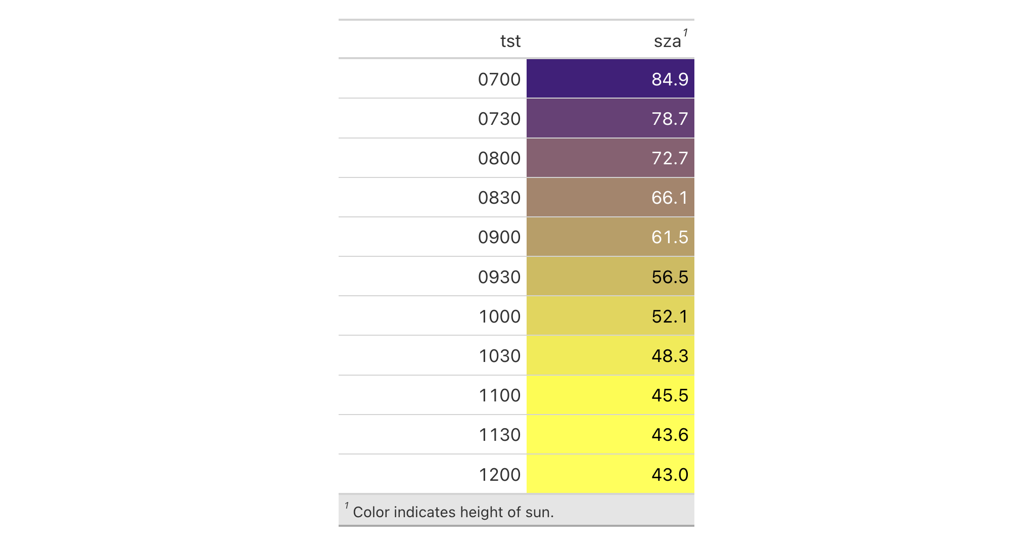
Let's use a small portion of the sza dataset to create a gt table.
Add footnotes to the column labels with tab_footnote() and
cells_column_labels() in locations.
sza |>
  dplyr::filter(
    latitude == 20 & month == "jan" &
      !is.na(sza)
  ) |>
  dplyr::select(-latitude, -month) |>
  gt() |>
  tab_footnote(
    footnote = "True solar time.",
    locations = cells_column_labels(
      columns = tst
    )
  ) |>
  tab_footnote(
    footnote = "Solar zenith angle.",
    locations = cells_column_labels(
      columns = sza
    )
  )

Function ID
8-15
Function Introduced
v0.2.0.5 (March 31, 2020)
See Also
Other location helper functions:
cells_body(),
cells_column_spanners(),
cells_footnotes(),
cells_grand_summary(),
cells_row_groups(),
cells_source_notes(),
cells_stub(),
cells_stub_grand_summary(),
cells_stub_summary(),
cells_stubhead(),
cells_summary(),
cells_title(),
location-helper
Location helper for targeting the column spanners
Description
cells_column_spanners() is used to target the cells that contain the table
column spanners. This is useful when applying a footnote with
tab_footnote() or adding custom style with tab_style(). The function is
expressly used in each of those functions' locations argument. The
'column_spanners' location is generated by one or more uses of
tab_spanner() or tab_spanner_delim().
Usage
cells_column_spanners(spanners = everything(), levels = NULL)cells_column_spanners(spanners = everything(), levels = NULL)
Arguments
spanners |
Specification of spanner IDs
The spanners to which targeting operations are constrained. Can either be a
series of spanner ID values provided in |
levels |
*Specification of the spanner levels *
The existing spanner levels (1, 2, ...) to which targeting operations are constrained. Use NULL to refer to all existing levels. |
Value
A list object with the classes cells_column_spanners and
location_cells.
Examples
Use the exibble dataset to create a gt table. We'll add a spanner
column label over three columns (date, time, and datetime) with
tab_spanner(). The spanner column label can be styled with tab_style() by
using the cells_column_spanners() function in locations. In this example,
we are making the text of the column spanner label appear as bold.
exibble |>
  dplyr::select(-fctr, -currency, -group) |>
  gt(rowname_col = "row") |>
  tab_spanner(
    label = "dates and times",
    columns = c(date, time, datetime),
    id = "dt"
  ) |>
  tab_style(
    style = cell_text(weight = "bold"),
    locations = cells_column_spanners(spanners = "dt")
  )

Use the exibble dataset to create a gt table. We'll add two spanners
for the column combinations of (num, char) and time related columns
(time and datetime). Furthermore we add another level of spanners with
a column label over all date- and time related columns (date, time, and
datetime). We want all spanner labels with "time" in their name to be bold.
Additionally we want the text to be red of the spanner that is both time-
related and on level 1.
exibble |>
  dplyr::select(-fctr, -currency, -group) |>
  gt(rowname_col = "row") |>
  tab_spanner(
    label = "time related cols",
    columns = c(datetime, time)
  ) |>
  tab_spanner(
    label = "num and char",
    columns = c(num, char)
  ) |>
  tab_spanner(
    label = "date and time cols",
    columns = c(date, time, datetime)
  ) |>
  tab_style(
    style = cell_text(weight = "bold"),
    locations = cells_column_spanners(spanners = tidyselect::contains("time"))
  ) |>
  tab_style(
    style = cell_text(color = "red"),
    locations = cells_column_spanners(
      spanners = tidyselect::contains("time"),
      levels = 1
    )
  )

Function ID
8-14
Function Introduced
v0.2.0.5 (March 31, 2020)
See Also
Other location helper functions:
cells_body(),
cells_column_labels(),
cells_footnotes(),
cells_grand_summary(),
cells_row_groups(),
cells_source_notes(),
cells_stub(),
cells_stub_grand_summary(),
cells_stub_summary(),
cells_stubhead(),
cells_summary(),
cells_title(),
location-helper
Location helper for targeting the footnotes
Description
cells_footnotes() is used to target all footnotes in the
footer section of the table. This is useful for adding custom styles to the
footnotes with tab_style() (using the locations argument). The
'footnotes' location is generated by one or more uses of tab_footnote().
This location helper function cannot be used for the locations argument of
tab_footnote() and doing so will result in a warning (with no change made
to the table).
Usage
cells_footnotes()cells_footnotes()
Value
A list object with the classes cells_footnotes and
location_cells.
Examples
Using a subset of the sza dataset, let's create a gt table. We'd like
to color the sza column so that's done with the data_color() function. We
can add a footnote with tab_footnote() and we can also style the
footnotes section. The styling is done with tab_style() and
locations = cells_footnotes().
sza |>
  dplyr::filter(
    latitude == 20 &
      month == "jan" &
      !is.na(sza)
  ) |>
  dplyr::select(-latitude, -month) |>
  gt() |>
  data_color(
    columns = sza,
    palette = c("white", "yellow", "navyblue"),
    domain = c(0, 90)
  ) |>
  tab_footnote(
    footnote = "Color indicates height of sun.",
    locations = cells_column_labels(columns = sza)
  ) |>
  tab_options(table.width = px(320)) |>
  tab_style(
    style = list(
      cell_text(size = "smaller"),
      cell_fill(color = "gray90")
      ),
    locations = cells_footnotes()
  )
Function ID
8-23
Function Introduced
v0.3.0 (May 12, 2021)
See Also
Other location helper functions:
cells_body(),
cells_column_labels(),
cells_column_spanners(),
cells_grand_summary(),
cells_row_groups(),
cells_source_notes(),
cells_stub(),
cells_stub_grand_summary(),
cells_stub_summary(),
cells_stubhead(),
cells_summary(),
cells_title(),
location-helper
Location helper for targeting cells in a grand summary
Description
cells_grand_summary() is used to target the cells in a grand
summary and it is useful when applying a footnote with tab_footnote() or
adding custom styles with tab_style(). The function is expressly used in
each of those functions' locations argument. The 'grand_summary' location
is generated by grand_summary_rows().
Usage
cells_grand_summary(columns = everything(), rows = everything())cells_grand_summary(columns = everything(), rows = everything())
Arguments
columns |
Columns to target
The columns to which targeting operations are constrained. Can either
be a series of column names provided in |
rows |
Rows to target
In conjunction with |
Value
A list object with the classes cells_grand_summary and
location_cells.
Targeting cells with columns and rows
Targeting of grand summary cells is done through the columns and rows
arguments. The columns argument allows us to target a subset of grand
summary cells contained in the resolved columns. We say resolved because
aside from declaring column names in c() (with bare column names or names
in quotes) we can use tidyselect-style expressions. This can be as basic
as supplying a select helper like starts_with(), or, providing a more
complex incantation like
where(~ is.numeric(.x) & max(.x, na.rm = TRUE) > 1E6)
which targets numeric columns that have a maximum value greater than
1,000,000 (excluding any NAs from consideration).
Once the columns are targeted, we may also target the rows of the grand
summary. Grand summary cells in the stub will have ID values that can be used
much like column names in the columns-targeting scenario. We can use
simpler tidyselect-style expressions (the select helpers should work well
here) and we can use quoted row identifiers in c(). It's also possible to
use row indices (e.g., c(3, 5, 6)) that correspond to the row number of a
grand summary row.
Examples
Use a portion of the countrypops dataset to create a gt table. Add
some styling to a grand summary cells with tab_style() and
cells_grand_summary() in the locations argument.
countrypops |>
  dplyr::filter(country_name == "Spain", year < 1970) |>
  dplyr::select(-contains("country")) |>
  gt(rowname_col = "year") |>
  fmt_number(
    columns = population,
    decimals = 0
  ) |>
  grand_summary_rows(
    columns = population,
    fns = change ~ max(.) - min(.),
    fmt = ~ fmt_integer(.)
  ) |>
  tab_style(
    style = list(
      cell_text(style = "italic"),
      cell_fill(color = "lightblue")
    ),
    locations = cells_grand_summary(
      columns = population,
      rows = 1
    )
  )

Function ID
8-20
Function Introduced
v0.2.0.5 (March 31, 2020)
See Also
Other location helper functions:
cells_body(),
cells_column_labels(),
cells_column_spanners(),
cells_footnotes(),
cells_row_groups(),
cells_source_notes(),
cells_stub(),
cells_stub_grand_summary(),
cells_stub_summary(),
cells_stubhead(),
cells_summary(),
cells_title(),
location-helper
Location helper for targeting row groups
Description
cells_row_groups() is used to target the table's row groups
when applying a footnote with tab_footnote() or adding custom style with
tab_style(). The function is expressly used in each of those functions'
locations argument. The 'row_groups' location can be generated by the
specifying a groupname_col in gt(), by introducing grouped data to gt()
(via dplyr::group_by()), or, by specifying groups with tab_row_group().
Usage
cells_row_groups(groups = everything())cells_row_groups(groups = everything())
Arguments
groups |
Specification of row group IDs
The row groups to which targeting operations are constrained. Can either be
a series of row group ID values provided in |
Value
A list object with the classes cells_row_groups and
location_cells.
Targeting cells with groups
By default groups is set to everything(), which means that all available
groups will be considered. Providing the ID values (in quotes) of row groups
in c() will serve to constrain the targeting to that subset of groups.
Examples
Let's use a summarized version of the pizzaplace dataset to create a
gt table with grouped data. Add a summary with summary_rows() and then
add a footnote to the "peppr_salami" row group label with tab_footnote();
the targeting is done with cells_row_groups() in the locations argument.
pizzaplace |>
  dplyr::filter(name %in% c("soppressata", "peppr_salami")) |>
  dplyr::group_by(name, size) |>
  dplyr::summarize(`Pizzas Sold` = dplyr::n(), .groups = "drop") |>
  gt(rowname_col = "size", groupname_col = "name") |>
  summary_rows(
    columns = `Pizzas Sold`,
    fns = list(label = "TOTAL", fn = "sum"),
    fmt = ~ fmt_integer(.)
  ) |>
  tab_footnote(
    footnote = "The Pepper-Salami.",
    cells_row_groups(groups = "peppr_salami")
  )

Function ID
8-16
Function Introduced
v0.2.0.5 (March 31, 2020)
See Also
Other location helper functions:
cells_body(),
cells_column_labels(),
cells_column_spanners(),
cells_footnotes(),
cells_grand_summary(),
cells_source_notes(),
cells_stub(),
cells_stub_grand_summary(),
cells_stub_summary(),
cells_stubhead(),
cells_summary(),
cells_title(),
location-helper
Location helper for targeting the source notes
Description
cells_source_notes() is used to target all source notes in the
footer section of the table. This is useful for adding custom styles to the
source notes with tab_style() (using the locations argument). The
'source_notes' location is generated by tab_source_note().
Usage
cells_source_notes()cells_source_notes()
Value
A list object with the classes cells_source_notes and
location_cells.
Examples
Let's use a subset of the gtcars dataset to create a gt table. Add a
source note (with tab_source_note()) and style the source notes section
inside tab_style() with locations = cells_source_notes().
gtcars |>
  dplyr::select(mfr, model, msrp) |>
  dplyr::slice(1:5) |>
  gt() |>
  tab_source_note(source_note = "From edmunds.com") |>
  tab_style(
    style = cell_text(
      color = "#A9A9A9",
      size = "small"
    ),
    locations = cells_source_notes()
  )

Function ID
8-24
Function Introduced
v0.3.0 (May 12, 2021)
See Also
Other location helper functions:
cells_body(),
cells_column_labels(),
cells_column_spanners(),
cells_footnotes(),
cells_grand_summary(),
cells_row_groups(),
cells_stub(),
cells_stub_grand_summary(),
cells_stub_summary(),
cells_stubhead(),
cells_summary(),
cells_title(),
location-helper
Location helper for targeting cells in the table stub
Description
cells_stub() is used to target the table's stub cells and it
is useful when applying a footnote with tab_footnote() or adding a custom
style with tab_style(). The function is expressly used in each of those
functions' locations argument. Here are several ways that a stub location
might be available in a gt table: (1) through specification of a
rowname_col in gt(), (2) by introducing a data frame with row names to
gt() with rownames_to_stub = TRUE, or (3) by using summary_rows() or
grand_summary_rows() with neither of the previous two conditions being
true.
Usage
cells_stub(rows = everything(), columns = NULL)cells_stub(rows = everything(), columns = NULL)
Arguments
rows |
Rows to target
The rows to which targeting operations are constrained. The default
Numeric indices: A vector of row indices within Content-based targeting: A vector of content values within Select helpers: Use functions like Expressions: Filter expressions to target specific rows
(e.g., When using content-based targeting with multi-column stubs, the function
will search all stub columns for matching values unless specific |
columns |
Stub columns to target
The stub columns to which targeting operations are constrained. By default
( |
Value
A list object with the classes cells_stub and location_cells.
Examples
Let's create a gt table using a transformed version of the sza
dataset. We'll color all of the month values in the table stub with
tab_style(), using cells_stub() in locations.
sza |>
  dplyr::filter(latitude == 20 & tst <= "1000") |>
  dplyr::select(-latitude) |>
  dplyr::filter(!is.na(sza)) |>
  tidyr::pivot_wider(
    names_from = "tst",
    values_from = sza,
    names_sort = TRUE
  ) |>
  gt(rowname_col = "month") |>
  sub_missing(missing_text = "") |>
  tab_style(
    style = list(
      cell_fill(color = "darkblue"),
      cell_text(color = "white")
      ),
    locations = cells_stub()
  )

For multi-column stubs, you can target specific columns. Here's an example with a table that has multiple stub columns:
dplyr::tibble(
  country = rep(c("USA", "Canada"), each = 3),
  region = rep(c("North", "South", "West"), 2),
  pop_2020 = c(5000, 3000, 2000, 4000, 3500, 1500),
  pop_2021 = c(5100, 3100, 2100, 4100, 3600, 1600)
) |>
  gt(rowname_col = c("country", "region")) |>
  tab_style(
    style = cell_fill(color = "lightblue"),
    locations = cells_stub(columns = "country", rows = 1:2)
  ) |>
  tab_style(
    style = cell_text(weight = "bold"),
    locations = cells_stub(columns = "region", rows = c(1, 3, 5))
  )

You can also use content-based targeting to target rows by their actual values rather than calculating row indices:
gtcars |>
  dplyr::select(mfr, model, year, hp, msrp) |>
  dplyr::slice(1:8) |>
  gt(rowname_col = c("mfr", "model")) |>
  tab_style(
    style = cell_fill(color = "lightcoral"),
    locations = cells_stub(rows = "Ford")  # Targets all Ford rows
  ) |>
  tab_style(
    style = cell_text(weight = "bold"),
    locations = cells_stub(rows = c("BMW", "Audi"), columns = "mfr")
  )

Function ID
8-17
Function Introduced
v0.2.0.5 (March 31, 2020)
See Also
Other location helper functions:
cells_body(),
cells_column_labels(),
cells_column_spanners(),
cells_footnotes(),
cells_grand_summary(),
cells_row_groups(),
cells_source_notes(),
cells_stub_grand_summary(),
cells_stub_summary(),
cells_stubhead(),
cells_summary(),
cells_title(),
location-helper
Location helper for targeting the stub cells in a grand summary
Description
cells_stub_grand_summary() is used to target the stub cells of
a grand summary and it is useful when applying a footnote with
tab_footnote() or adding custom styles with tab_style(). The function is
expressly used in each of those functions' locations argument. The
'stub_grand_summary' location is generated by grand_summary_rows().
Usage
cells_stub_grand_summary(rows = everything())cells_stub_grand_summary(rows = everything())
Arguments
rows |
Rows to target
We can specify which rows should be targeted. The default |
Value
A list object with the classes cells_stub_grand_summary and
location_cells.
Targeting grand summary stub cells with rows
Targeting the stub cells of a grand summary row is done through the rows
argument. Grand summary cells in the stub will have ID values that can be
used much like column names in the columns-targeting scenario. We can use
simpler tidyselect-style expressions (the select helpers should work well
here) and we can use quoted row identifiers in c(). It's also possible to
use row indices (e.g., c(3, 5, 6)) that correspond to the row number of a
grand summary row.
Examples
Use a portion of the countrypops dataset to create a gt table. Add
some styling to a grand summary stub cell with tab_style() and using
cells_stub_grand_summary() in the locations argument.
countrypops |>
  dplyr::filter(country_name == "Spain", year < 1970) |>
  dplyr::select(-contains("country")) |>
  gt(rowname_col = "year") |>
  fmt_number(
    columns = population,
    decimals = 0
  ) |>
  grand_summary_rows(
    columns = population,
    fns = list(change = ~max(.) - min(.)),
    fmt = ~ fmt_integer(.)
  ) |>
  tab_style(
    style = cell_text(weight = "bold", transform = "uppercase"),
    locations = cells_stub_grand_summary(rows = "change")
  )

Function ID
8-22
Function Introduced
v0.3.0 (May 12, 2021)
See Also
Other location helper functions:
cells_body(),
cells_column_labels(),
cells_column_spanners(),
cells_footnotes(),
cells_grand_summary(),
cells_row_groups(),
cells_source_notes(),
cells_stub(),
cells_stub_summary(),
cells_stubhead(),
cells_summary(),
cells_title(),
location-helper
Location helper for targeting the stub cells in a summary
Description
cells_stub_summary() is used to target the stub cells of
summary and it is useful when applying a footnote with tab_footnote() or
adding custom styles with tab_style(). The function is expressly used in
each of those functions' locations argument. The 'stub_summary' location is
generated by summary_rows().
Usage
cells_stub_summary(groups = everything(), rows = everything())cells_stub_summary(groups = everything(), rows = everything())
Arguments
groups |
Specification of row group IDs
The row groups to which targeting operations are constrained. Can either be
a series of row group ID values provided in |
rows |
Rows to target
In conjunction with |
Value
A list object with the classes cells_stub_summary and
location_cells.
Targeting summary stub cells with groups and rows
Targeting the stub cells of group summary rows is done through the groups
and rows arguments. By default groups is set to everything(), which means
that all available groups will be considered. Providing the ID values (in
quotes) of row groups in c() will serve to constrain the targeting to that
subset of groups.
Once the groups are targeted, we may also target the rows of the summary.
Summary cells in the stub will have ID values that can be used much like
column names in the columns-targeting scenario. We can use simpler
tidyselect-style expressions (the select helpers should work well here)
and we can use quoted row identifiers in c(). It's also possible to use row
indices (e.g., c(3, 5, 6)) that correspond to the row number of a summary
row in a row group (numbering restarts with every row group).
Examples
Use a portion of the countrypops dataset to create a gt table. Add
some styling to the summary data stub cells with tab_style() and
cells_stub_summary() in the locations argument.
countrypops |>
  dplyr::filter(country_name == "Japan", year < 1970) |>
  dplyr::select(-contains("country")) |>
  dplyr::mutate(decade = paste0(substr(year, 1, 3), "0s")) |>
  gt(
    rowname_col = "year",
    groupname_col = "decade"
  ) |>
  fmt_integer(columns = population) |>
  summary_rows(
    groups = "1960s",
    columns = population,
    fns = list("min", "max"),
    fmt = ~ fmt_integer(.)
  ) |>
  tab_style(
    style = list(
      cell_text(
        weight = "bold",
        transform = "capitalize"
      ),
      cell_fill(
        color = "lightblue",
        alpha = 0.5
      )
    ),
    locations = cells_stub_summary(
      groups = "1960s"
    )
  )

Function ID
8-21
Function Introduced
v0.3.0 (May 12, 2021)
See Also
Other location helper functions:
cells_body(),
cells_column_labels(),
cells_column_spanners(),
cells_footnotes(),
cells_grand_summary(),
cells_row_groups(),
cells_source_notes(),
cells_stub(),
cells_stub_grand_summary(),
cells_stubhead(),
cells_summary(),
cells_title(),
location-helper
Location helper for targeting the table stubhead cell
Description
cells_stubhead() is used to target the table stubhead location
when applying a footnote with tab_footnote() or adding custom style with
tab_style(). The function is expressly used in each of those functions'
locations argument. The 'stubhead' location is always present alongside the
'stub' location.
Usage
cells_stubhead()cells_stubhead()
Value
A list object with the classes cells_stubhead and location_cells.
Examples
Using a summarized version of the pizzaplace dataset, let's create a
gt table. Add a stubhead label with tab_stubhead() and then style it
with tab_style() in conjunction with the use of cells_stubhead() in the
locations argument.
pizzaplace |>
  dplyr::mutate(month = as.numeric(substr(date, 6, 7))) |>
  dplyr::group_by(month, type) |>
  dplyr::summarize(sold = dplyr::n(), .groups = "drop") |>
  dplyr::filter(month %in% 1:2) |>
  gt(rowname_col = "type") |>
  tab_stubhead(label = "type") |>
  tab_style(
    style = cell_fill(color = "lightblue"),
    locations = cells_stubhead()
  )

Function ID
8-13
Function Introduced
v0.2.0.5 (March 31, 2020)
See Also
Other location helper functions:
cells_body(),
cells_column_labels(),
cells_column_spanners(),
cells_footnotes(),
cells_grand_summary(),
cells_row_groups(),
cells_source_notes(),
cells_stub(),
cells_stub_grand_summary(),
cells_stub_summary(),
cells_summary(),
cells_title(),
location-helper
Location helper for targeting group summary cells
Description
cells_summary() is used to target the cells in a group summary and it is
useful when applying a footnote with tab_footnote() or adding a custom
style with tab_style(). The function is expressly used in each of those
functions' locations argument. The 'summary' location is generated by
summary_rows().
Usage
cells_summary( groups = everything(), columns = everything(), rows = everything() )cells_summary( groups = everything(), columns = everything(), rows = everything() )
Arguments
groups |
Specification of row group IDs
The row groups to which targeting operations are constrained. This aids in
targeting the summary rows that reside in certain row groups. Can either be
a series of row group ID values provided in |
columns |
Columns to target
The columns to which targeting operations are constrained. Can either
be a series of column names provided in |
rows |
Rows to target
In conjunction with |
Value
A list object with the classes cells_summary and location_cells.
Targeting cells with columns, rows, and groups
Targeting of summary cells is done through the groups, columns, and
rows arguments. By default groups is set to everything(), which means
that all available groups will be considered. Providing the ID values (in
quotes) of row groups in c() will serve to constrain the targeting to that
subset of groups.
The columns argument allows us to target a subset of summary
cells contained in the resolved columns. We say resolved because aside from
declaring column names in c() (with bare column names or names in quotes)
we can use tidyselect-style expressions. This can be as basic as
supplying a select helper like starts_with(), or, providing a more complex
incantation like
where(~ is.numeric(.x) & max(.x, na.rm = TRUE) > 1E6)
which targets numeric columns that have a maximum value greater than
1,000,000 (excluding any NAs from consideration).
Once the groups and columns are targeted, we may also target the rows of
the summary. Summary cells in the stub will have ID values that can be used
much like column names in the columns-targeting scenario. We can use
simpler tidyselect-style expressions (the select helpers should work well
here) and we can use quoted row identifiers in c(). It's also possible to
use row indices (e.g., c(3, 5, 6)) that correspond to the row number of a
summary row in a row group (numbering restarts with every row group).
Examples
Use a portion of the countrypops dataset to create a gt table. Add
some styling to the summary data cells with tab_style(), using
cells_summary() in the locations argument.
countrypops |>
  dplyr::filter(country_name == "Japan", year < 1970) |>
  dplyr::select(-contains("country")) |>
  dplyr::mutate(decade = paste0(substr(year, 1, 3), "0s")) |>
  gt(
    rowname_col = "year",
    groupname_col = "decade"
  ) |>
  fmt_number(
    columns = population,
    decimals = 0
  ) |>
  summary_rows(
    groups = "1960s",
    columns = population,
    fns = list("min", "max"),
    fmt = ~ fmt_integer(.)
  ) |>
  tab_style(
    style = list(
      cell_text(style = "italic"),
      cell_fill(color = "lightblue")
    ),
    locations = cells_summary(
      groups = "1960s",
      columns = population,
      rows = 1
    )
  ) |>
  tab_style(
    style = list(
      cell_text(style = "italic"),
      cell_fill(color = "lightgreen")
    ),
    locations = cells_summary(
      groups = "1960s",
      columns = population,
      rows = 2
    )
  )

Function ID
8-19
Function Introduced
v0.2.0.5 (March 31, 2020)
See Also
Other location helper functions:
cells_body(),
cells_column_labels(),
cells_column_spanners(),
cells_footnotes(),
cells_grand_summary(),
cells_row_groups(),
cells_source_notes(),
cells_stub(),
cells_stub_grand_summary(),
cells_stub_summary(),
cells_stubhead(),
cells_title(),
location-helper
Location helper for targeting the table title and subtitle
Description
cells_title() is used to target the table title or subtitle
when applying a footnote with tab_footnote() or adding custom style with
tab_style(). The function is expressly used in each of those functions'
locations argument. The header location where the title and optionally the
subtitle reside is generated by the tab_header() function.
Usage
cells_title(groups = c("title", "subtitle"))cells_title(groups = c("title", "subtitle"))
Arguments
groups |
Specification of groups
We can either specify |
Value
A list object of classes cells_title and location_cells.
Examples
Use a subset of the sp500 dataset to create a small gt table. Add a
header with a title, and then add a footnote to the title with
tab_footnote() and cells_title() (in locations).
sp500 |>
  dplyr::filter(date >= "2015-01-05" & date <= "2015-01-10") |>
  dplyr::select(-c(adj_close, volume, high, low)) |>
  gt() |>
  tab_header(title = "S&P 500") |>
  tab_footnote(
    footnote = "All values in USD.",
    locations = cells_title(groups = "title")
  )

Function ID
8-12
Function Introduced
v0.2.0.5 (March 31, 2020)
See Also
Other location helper functions:
cells_body(),
cells_column_labels(),
cells_column_spanners(),
cells_footnotes(),
cells_grand_summary(),
cells_row_groups(),
cells_source_notes(),
cells_stub(),
cells_stub_grand_summary(),
cells_stub_summary(),
cells_stubhead(),
cells_summary(),
location-helper
Add one or more columns to a gt table
Description
We can add new columns to a table with cols_add() and it works quite a bit
like dplyr::mutate() does. The idea is that you supply name-value pairs
where the name is the new column name and the value part describes the data
that will go into the column. The latter can: (1) be a vector where the
length of the number of rows in the data table, (2) be a single value
(which will be repeated all the way down), or (3) involve other columns in
the table (as they represent vectors of the correct length). The new columns
are added to the end of the column series by default but can instead be added
internally by using either the .before or .after arguments. If entirely
empty (i.e., all NA) columns need to be added, you can use any of the NA
types (e.g., NA, NA_character_, NA_real_, etc.) for such columns.
Usage
cols_add(.data, ..., .before = NULL, .after = NULL)cols_add(.data, ..., .before = NULL, .after = NULL)
Arguments
.data |
The gt table or gt group data object
This is the gt table object that is commonly created through use of the
OR
This is the gt group object that is commonly created through use of the
|
... |
Cell data assignments
Expressions for the assignment of cell values to the new columns.
Name-value pairs, in the form of |
.before, .after
|
Column used as anchor
A single column-resolving expression or column index can be given to either
|
Value
An object of class gt_tbl.
Targeting the column for insertion with .before or .after
The targeting of a column for insertion is done through the .before or
.after arguments (only one of these options should be used). While
tidyselect-style expressions or indices can used to target a column, it's
advised that a single column name be used. This is to avoid the possibility
of inadvertently resolving multiple columns (since the requirement is for a
single column).
Examples
Let's take a subset of the exibble dataset and make a simple gt table
with it (using the row column for labels in the stub). We'll add a single
column to the right of all the existing columns and call it country. This
new column needs eight values and these will be supplied when using
cols_add().
exibble |>
  dplyr::select(num, char, datetime, currency, group) |>
  gt(rowname_col = "row") |>
  cols_add(
    country = c("TL", "PY", "GL", "PA", "MO", "EE", "CO", "AU")
  )

We can add multiple columns with a single use of cols_add(). The columns
generated can be formatted and otherwise manipulated just as any column could
be in a gt table. The following example extends the first one by adding
more columns and immediately using them in various function calls like
fmt_flag() and fmt_units().
exibble |>
  dplyr::select(num, char, datetime, currency, group) |>
  gt(rowname_col = "row") |>
  cols_add(
    country = c("TL", "PY", "GL", "PA", "MO", "EE", "CO", "AU"),
    empty = NA_character_,
    units = c(
      "k m s^-2", "N m^-2", "degC", "m^2 kg s^-2",
      "m^2 kg s^-3", "/s", "A s", "m^2 kg s^-3 A^-1"
    ),
    big_num = num ^ 3
  ) |>
  fmt_flag(columns = country) |>
  sub_missing(columns = empty, missing_text = "") |>
  fmt_units(columns = units) |>
  fmt_scientific(columns = big_num)

In this table generated from a portion of the towny dataset, we add two
new columns (land_area and density) through a single use of cols_add().
The new land_area column is a conversion of land area from square
kilometers to square miles and the density column is calculated by through
division of population_2021 by that new land_area column. We hide the
now unneeded land_area_km2 with cols_hide() and also perform some column
labeling and adjustments to column widths with cols_label() and
cols_width().
towny |>
  dplyr::select(name, population_2021, land_area_km2) |>
  dplyr::filter(population_2021 > 100000) |>
  dplyr::slice_max(population_2021, n = 10) |>
  gt() |>
  cols_add(
    land_area = land_area_km2 / 2.58998811,
    density = population_2021 / land_area
  ) |>
  fmt_integer() |>
  cols_hide(columns = land_area_km2) |>
  cols_label(
    population_2021 = "Population",
    density = "Density, {{*persons* / sq mi}}",
    land_area ~ "Area, {{mi^2}}"
  ) |>
  cols_width(everything() ~ px(120))

It's possible to start with an empty table (i.e., no columns and no rows) and
add one or more columns to that. You can, for example, use dplyr::tibble()
or data.frame() to create a completely empty table. The first cols_add()
call for an empty table can have columns of arbitrary length but subsequent
uses of cols_add() must adhere to the rule of new columns being the same
length as existing.
dplyr::tibble() |>
  gt() |>
  cols_add(
    num = 1:5,
    chr = vec_fmt_spelled_num(1:5)
  )

Tables can contain no rows, yet have columns. In the following example, we'll
create a zero-row table with three columns (num, chr, and ext) and
perform the same cols_add()-based addition of two columns of data. This is
another case where the function allows for arbitrary-length columns (since
always adding zero-length columns is impractical). Furthermore, here we can
reference columns that already exist (num and chr) and add values to
them.
dplyr::tibble(
  num = numeric(0),
  chr = character(0),
  ext = character(0)
) |>
  gt() |>
  cols_add(
    num = 1:5,
    chr = vec_fmt_spelled_num(1:5)
  )

We should note that the ext column did not receive any values from
cols_add() but the table was expanded to having five rows nonetheless. So,
each cell of ext was by necessity filled with an NA value.
Function ID
5-7
Function Introduced
v0.10.0 (October 7, 2023)
See Also
Other column modification functions:
cols_align(),
cols_align_decimal(),
cols_hide(),
cols_label(),
cols_label_with(),
cols_merge(),
cols_merge_n_pct(),
cols_merge_range(),
cols_merge_uncert(),
cols_move(),
cols_move_to_end(),
cols_move_to_start(),
cols_nanoplot(),
cols_unhide(),
cols_units(),
cols_width()
Set the alignment of columns
Description
The individual alignments of columns (which includes the column labels and
all of their data cells) can be modified. We have the option to align text to
the left, the center, and the right. In a less explicit manner, we can
allow gt to automatically choose the alignment of each column based on
the data type (with the auto option).
Usage
cols_align( data, align = c("auto", "left", "center", "right"), columns = everything() )cols_align( data, align = c("auto", "left", "center", "right"), columns = everything() )
Arguments
data |
The gt table or gt group data object
This is the gt table object that is commonly created through use of the
OR
This is the gt group object that is commonly created through use of the
|
align |
Alignment type
This can be any of |
columns |
Columns to target
The columns for which the alignment should be applied. Can either be a
series of column names provided in |
Details
When you create a gt table object using gt(), automatic alignment of
column labels and their data cells is performed. By default, left-alignment
is applied to columns of class character, Date, or POSIXct;
center-alignment is for columns of class logical, factor, or list; and
right-alignment is used for the numeric and integer columns.
Value
An object of class gt_tbl.
Examples
Let's use countrypops to create a small gt table. We can change the
alignment of the population column with cols_align(). In this example,
the label and body cells of population will be aligned to the left.
countrypops |>
  dplyr::select(-contains("code")) |>
  dplyr::filter(
    country_name == "San Marino",
    year %in% 2017:2021
  ) |>
  gt(
    rowname_col = "year",
    groupname_col = "country_name"
  ) |>
  cols_align(
    align = "left",
    columns = population
  )

Function ID
5-1
Function Introduced
v0.2.0.5 (March 31, 2020)
See Also
Other column modification functions:
cols_add(),
cols_align_decimal(),
cols_hide(),
cols_label(),
cols_label_with(),
cols_merge(),
cols_merge_n_pct(),
cols_merge_range(),
cols_merge_uncert(),
cols_move(),
cols_move_to_end(),
cols_move_to_start(),
cols_nanoplot(),
cols_unhide(),
cols_units(),
cols_width()
Align all numeric values in a column along the decimal mark
Description
For numeric columns that contain values with decimal portions, it is
sometimes useful to have them lined up along the decimal mark for easier
readability. We can do this with cols_align_decimal() and provide any
number of columns (the function will skip over columns that don't require
this type of alignment).
Usage
cols_align_decimal(data, columns = everything(), dec_mark = ".", locale = NULL)cols_align_decimal(data, columns = everything(), dec_mark = ".", locale = NULL)
Arguments
data |
The gt table or gt group data object
This is the gt table object that is commonly created through use of the
OR
This is the gt group object that is commonly created through use of the
|
columns |
Columns to target
The columns for which decimal alignment should be applied. Can either be a
series of column names provided in |
dec_mark |
Decimal mark
The character used as a decimal mark in the numeric values to be aligned.
If a locale value was used when formatting the numeric values then |
locale |
Locale identifier
An optional locale identifier that can be used to obtain the type of
decimal mark used in the numeric values to be aligned (according to the
locale's formatting rules). Examples include |
Value
An object of class gt_tbl.
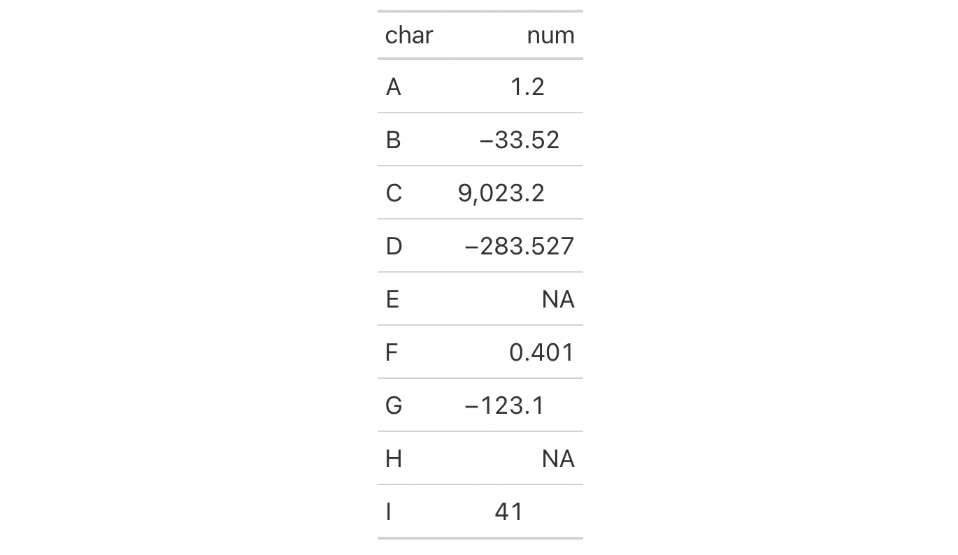
Examples
Let's put together a two-column table to create a gt table. The first
column char just contains letters whereas the second column, num, has a
collection of numbers and NA values. We could format the numbers with
fmt_number() and elect to drop the trailing zeros past the decimal mark
with drop_trailing_zeros = TRUE. This can leave formatted numbers that are
hard to scan through because the decimal mark isn't fixed horizontally. We
could remedy this and align the numbers by the decimal mark with
cols_align_decimal().
dplyr::tibble(
  char = LETTERS[1:9],
  num = c(1.2, -33.52, 9023.2, -283.527, NA, 0.401, -123.1, NA, 41)
) |>
  gt() |>
  fmt_number(
    columns = num,
    decimals = 3,
    drop_trailing_zeros = TRUE
  ) |>
  cols_align_decimal()
Function ID
5-2
Function Introduced
v0.8.0 (November 16, 2022)
See Also
Other column modification functions:
cols_add(),
cols_align(),
cols_hide(),
cols_label(),
cols_label_with(),
cols_merge(),
cols_merge_n_pct(),
cols_merge_range(),
cols_merge_uncert(),
cols_move(),
cols_move_to_end(),
cols_move_to_start(),
cols_nanoplot(),
cols_unhide(),
cols_units(),
cols_width()
Hide one or more columns
Description
cols_hide() allows us to hide one or more columns from
appearing in the final output table. While it's possible and often desirable
to omit columns from the input table data before introduction to gt(),
there can be cases where the data in certain columns is useful (as a column
reference during formatting of other columns) but the final display of those
columns is not necessary.
Usage
cols_hide(data, columns)cols_hide(data, columns)
Arguments
data |
The gt table or gt group data object
This is the gt table object that is commonly created through use of the
OR
This is the gt group object that is commonly created through use of the
|
columns |
Columns to target
The columns to hide in the output display table. Can either be a series of
column names provided in |
Details
The hiding of columns is internally a rendering directive, so, all columns
that are 'hidden' are still accessible and useful in any expression provided
to a rows argument. Furthermore, cols_hide() (as with many gt
functions) can be placed anywhere in a pipeline of gt function calls
(acting as a promise to hide columns when the timing is right). However,
there's perhaps greater readability when placing this call closer to the end
of such a pipeline. cols_hide() quietly changes the visible state of a
column (much like cols_unhide()) and doesn't yield warnings or messages
when changing the state of already-invisible columns.
Value
An object of class gt_tbl. data will be unaltered if columns is
not supplied.
Examples
Let's use a small portion of the countrypops dataset to create a gt
table. We can hide the country_code_2 and country_code_3 columns with the
cols_hide() function.
countrypops |>
  dplyr::filter(
    country_name == "Egypt",
    year %in% 2017:2021
  ) |>
  gt() |>
  cols_hide(columns = c(country_code_2, country_code_3))

Using another countrypops-based gt table, we can use the population
column to provide the conditional placement of footnotes. Then, we'll hide
that column along with the country_code_3 column. Note that the order of
cols_hide() and tab_footnote() has no effect on the final display of the
table.
countrypops |>
  dplyr::filter(
    country_name == "Pakistan",
    year %in% 2017:2021
  ) |>
  gt() |>
  cols_hide(columns = c(country_code_3, population)) |>
  tab_footnote(
    footnote = "Population above 220,000,000.",
    locations = cells_body(
      columns = year,
      rows = population > 220E6
    )
  )

Function ID
5-12
Function Introduced
v0.2.0.5 (March 31, 2020)
See Also
cols_unhide() to perform the inverse operation.
Other column modification functions:
cols_add(),
cols_align(),
cols_align_decimal(),
cols_label(),
cols_label_with(),
cols_merge(),
cols_merge_n_pct(),
cols_merge_range(),
cols_merge_uncert(),
cols_move(),
cols_move_to_end(),
cols_move_to_start(),
cols_nanoplot(),
cols_unhide(),
cols_units(),
cols_width()
Relabel one or more columns
Description
Column labels can be modified from their default values (the names of the
columns from the input table data). When you create a gt table object
using gt(), column names effectively become the column labels. While this
serves as a good first approximation, column names as label defaults aren't
often as appealing in a gt table as the option for custom column labels.
cols_label() provides the flexibility to relabel one or more columns and
we even have the option to use md() or html() for rendering column labels
from Markdown or using HTML.
Usage
cols_label(.data, ..., .list = list2(...), .fn = NULL, .process_units = NULL)cols_label(.data, ..., .list = list2(...), .fn = NULL, .process_units = NULL)
Arguments
.data |
The gt table or gt group data object
This is the gt table object that is commonly created through use of the
OR
This is the gt group object that is commonly created through use of the
|
... |
Column label assignments
Expressions for the assignment of column labels for the table columns in
|
.list |
Alternative to
Allows for the use of a list as an input alternative to |
.fn |
Function to apply
An option to specify a function that will be applied to all of the provided label values. |
.process_units |
Option to process any available units throughout
Should your column text contain text that is already in gt's units
notation (and, importantly, is surrounded by |
Value
An object of class gt_tbl.
A note on column names and column labels
It's important to note that while columns can be freely relabeled, we
continue to refer to columns by their original column names. Column names in
a tibble or data frame must be unique whereas column labels in gt have
no requirement for uniqueness (which is useful for labeling columns as, say,
measurement units that may be repeated several times—usually under
different spanner labels). Thus, we can still easily distinguish
between columns in other gt function calls (e.g., in all of the
fmt*() functions) even though we may lose distinguishability between column
labels once they have undergone relabeling.
Incorporating units with gt's units notation
Measurement units are often seen as part of column labels and indeed it can
be much more straightforward to include them here rather than using other
devices to make readers aware of units for specific columns. The gt
package offers the function cols_units() to apply units to various columns
with an interface that's similar to that of this function. However, it is
also possible to define units here along with the column label, obviating the
need for pattern syntax that joins the two text components. To do this, we
have to surround the portion of text in the label that corresponds to the
units definition with "{{"/"}}".
Now that we know how to mark text for units definition, we know need to know how to write proper units with the notation. Such notation uses a succinct method of writing units and it should feel somewhat familiar though it is particular to the task at hand. Each unit is treated as a separate entity (parentheses and other symbols included) and the addition of subscript text and exponents is flexible and relatively easy to formulate. This is all best shown with a few examples:
-
"m/s"and"m / s"both render as"m/s" -
"m s^-1"will appear with the"-1"exponent intact -
"m /s"gives the same result, as"/<unit>"is equivalent to"<unit>^-1" -
"E_h"will render an"E"with the"h"subscript -
"t_i^2.5"provides atwith an"i"subscript and a"2.5"exponent -
"m[_0^2]"will use overstriking to set both scripts vertically -
"g/L %C6H12O6%"uses a chemical formula (enclosed in a pair of"%"characters) as a unit partial, and the formula will render correctly with subscripted numbers -
Common units that are difficult to write using ASCII text may be implicitly converted to the correct characters (e.g., the
"u"in"ug","um","uL", and"umol"will be converted to the Greek mu symbol;"degC"and"degF"will render a degree sign before the temperature unit) -
We can transform shorthand symbol/unit names enclosed in
":"(e.g.,":angstrom:",":ohm:", etc.) into proper symbols -
Greek letters can added by enclosing the letter name in
":"; you can use lowercase letters (e.g.,":beta:",":sigma:", etc.) and uppercase letters too (e.g.,":Alpha:",":Zeta:", etc.) -
The components of a unit (unit name, subscript, and exponent) can be fully or partially italicized/emboldened by surrounding text with
"*"or"**"
Examples
Let's use a portion of the countrypops dataset to create a gt table.
We can relabel all the table's columns with the cols_label() function to
improve its presentation. In this simple case we are supplying the name of
the column on the left-hand side, and the label text on the right-hand side.
countrypops |>
  dplyr::select(-contains("code")) |>
  dplyr::filter(
    country_name == "Uganda",
    year %in% 2017:2021
  ) |>
  gt() |>
  cols_label(
    country_name = "Name",
    year = "Year",
    population = "Population"
  )

Using the countrypops dataset again, we label columns similarly to before
but this time making the column labels be bold through Markdown formatting
(with the md() helper function). It's possible here to use either a = or
a ~ between the column name and the label text.
countrypops |>
  dplyr::select(-contains("code")) |>
  dplyr::filter(
    country_name == "Uganda",
    year %in% 2017:2021
  ) |>
  gt() |>
  cols_label(
    country_name = md("**Name**"),
    year = md("**Year**"),
    population ~ md("**Population**")
  )

With a select portion of the metro dataset, let's create a small gt
table with three columns. Within cols_label() we'd like to provide column
labels that contain line breaks. For that, we can use <br> to indicate
where the line breaks should be. We also need to use the md() helper
function to signal to gt that this text should be interpreted as
Markdown. Instead of calling md() on each of labels as before, we can more
conveniently use the .fn argument and provide the bare function there (it
will be applied to each label defined in the cols_label() call).
metro |>
  dplyr::select(name, lines, passengers, connect_other) |>
  dplyr::slice_max(passengers, n = 10) |>
  gt() |>
  cols_hide(columns = passengers) |>
  cols_label(
    name = "Name of<br>Metro Station",
    lines = "Metro<br>Lines",
    connect_other = "Train<br>Services",
    .fn = md
  )

Using a subset of the towny dataset, we can create an interesting gt
table. First, only certain columns are selected from the dataset, some
filtering of rows is done, rows are sorted, and then only the first 10 rows
are kept. After the data is introduced to gt(), we then apply some spanner
labels using two calls of tab_spanner(). Below those spanners, we want to
label the columns by the years of interest. Using cols_label() and select
expressions on the left side of the formulas, we can easily relabel multiple
columns with common label text. Note that we cannot use an = sign in any of
the expressions within cols_label(); because the left-hand side is not a
single column name, we must use formula syntax (i.e., with the ~).
towny |>
  dplyr::select(
    name, ends_with("2001"), ends_with("2006"), matches("2001_2006")
  ) |>
  dplyr::filter(population_2001 > 100000) |>
  dplyr::slice_max(pop_change_2001_2006_pct, n = 10) |>
  gt() |>
  fmt_integer() |>
  fmt_percent(columns = matches("change"), decimals = 1) |>
  tab_spanner(label = "Population", columns = starts_with("population")) |>
  tab_spanner(label = "Density", columns = starts_with("density")) |>
  cols_label(
    ends_with("01") ~ "2001",
    ends_with("06") ~ "2006",
    matches("change") ~ md("Population Change,<br>2001 to 2006")
  ) |>
  cols_width(everything() ~ px(120))

Here's another table that uses the towny dataset. The big difference
compared to the previous gt table is that cols_label() as used here
incorporates unit notation text (within "{{"/"}}").
towny |>
  dplyr::select(
    name, population_2021, density_2021, land_area_km2, latitude, longitude
  ) |>
  dplyr::slice_max(population_2021, n = 10) |>
  gt() |>
  fmt_integer(columns = population_2021) |>
  fmt_number(
    columns = c(density_2021, land_area_km2),
    decimals = 1
  ) |>
  fmt_number(columns = latitude, decimals = 2) |>
  fmt_number(columns = longitude, decimals = 2, scale_by = -1) |>
  cols_label(
    starts_with("population") ~ "Population",
    starts_with("density") ~ "Density, {{*persons* km^-2}}",
    land_area_km2 ~ "Area, {{km^2}}",
    latitude ~ "Latitude, {{:degrees:N}}",
    longitude ~ "Longitude, {{:degrees:W}}"
  ) |>
  cols_width(everything() ~ px(120))

The illness dataset has units within the units column. They're
formatted in just the right way for gt too. Let's do some text
manipulation through dplyr::mutate() and some pivoting with
tidyr::pivot_longer() and tidyr::pivot_wider() in order to include the
units as part of the column names in the reworked table. These column names
are in a format where the units are included within "{{"/"}}", so, we can
use cols_label() with the .process_units = TRUE option to register the
measurement units. In addition to this, because there is a <br> included
(for a line break), we should use the .fn option and provide the md()
helper function (as a bare function name). This ensures that any line breaks
will materialize.
illness |>
  dplyr::mutate(test = paste0(test, ",<br>{{", units, "}}")) |>
  dplyr::slice_head(n = 8) |>
  dplyr::select(-c(starts_with("norm"), units)) |>
  tidyr::pivot_longer(
    cols = starts_with("day"),
    names_to = "day",
    names_prefix = "day_",
    values_to = "value"
  ) |>
  tidyr::pivot_wider(
    names_from = test,
    values_from = value
  ) |>
  gt(rowname_col = "day") |>
  tab_stubhead(label = "Day") |>
  cols_label(
    .fn = md,
    .process_units = TRUE
  ) |>
  cols_width(
    stub() ~ px(50),
    everything() ~ px(120)
  )

Function ID
5-4
Function Introduced
v0.2.0.5 (March 31, 2020)
See Also
Other column modification functions:
cols_add(),
cols_align(),
cols_align_decimal(),
cols_hide(),
cols_label_with(),
cols_merge(),
cols_merge_n_pct(),
cols_merge_range(),
cols_merge_uncert(),
cols_move(),
cols_move_to_end(),
cols_move_to_start(),
cols_nanoplot(),
cols_unhide(),
cols_units(),
cols_width()
Relabel columns with a function
Description
Column labels can be modified from their default values (the names of the
columns from the input table data). When you create a gt table object
using gt(), column names effectively become the column labels. While this
serves as a good first approximation, you may want to make adjustments so
that the columns names present better in the gt output table. The
cols_label_with() function allows for modification of column labels through
a supplied function. By default, the function will be invoked on all column
labels but this can be limited to a subset via the columns argument. With
the fn argument, we provide either a bare function name, a RHS formula
(with . representing the vector of column labels), or, an anonymous
function (e.g., function(x) tools::toTitleCase(x)).
Usage
cols_label_with(data, columns = everything(), fn)cols_label_with(data, columns = everything(), fn)
Arguments
data |
The gt table or gt group data object
This is the gt table object that is commonly created through use of the
OR
This is the gt group object that is commonly created through use of the
|
columns |
Columns to target
The columns for which the column-labeling operations should be applied. Can
either be a series of column names provided in |
fn |
Function to apply
The function or function call to be applied to the column labels. This can
take the form of a bare function (e.g., |
Value
An object of class gt_tbl.
A note on column names and column labels
It's important to note that while columns can be freely relabeled, we
continue to refer to columns by their original column names. Column names in
a tibble or data frame must be unique whereas column labels in gt have no
requirement for uniqueness (which is useful for labeling columns as, say,
measurement units that may be repeated several times—usually under
different spanner labels). Thus, we can still easily distinguish between
columns in other gt function calls (e.g., in all of the fmt*()
functions) even though we may lose distinguishability in column labels once
they have been relabeled.
Examples
Use a subset of the sp500 dataset to create a gt table. We want all
the column labels to be entirely capitalized versions of the default labels
but, instead of using cols_label() and rewriting each label manually in
capital letters we can use cols_label_with() and instruct it to apply the
toupper() function to all column labels.
sp500 |>
  dplyr::filter(
    date >= "2015-12-01" &
      date <= "2015-12-15"
  ) |>
  dplyr::select(-c(adj_close, volume)) |>
  gt() |>
  cols_label_with(fn = toupper)

Use the countrypops dataset to create a gt table. To improve the
presentation of the table, we are again going to change the default column
labels via function calls supplied within cols_label_with(). We can, if we
prefer, apply multiple types of column label changes in sequence with
multiple calls of cols_label_with(). Here, we use the make_clean_names()
functions from the janitor package and follow up with the removal of a
numeral with gsub().
countrypops |>
  dplyr::filter(year == 2021) |>
  dplyr::filter(grepl("^C", country_code_3)) |>
  dplyr::select(-country_code_2, -year) |>
  head(8) |>
  gt() |>
  cols_move_to_start(columns = country_code_3) |>
  fmt_integer(columns = population) |>
  cols_label_with(
    fn = ~ janitor::make_clean_names(., case = "title")
  ) |>
  cols_label_with(
    fn = ~ gsub("[0-9]", "", .)
  )

We can make a svelte gt table with the pizzaplace dataset. There are
ways to use one instance of cols_label_with() with multiple functions
called on the column labels. In the example, we use an anonymous function
call (with the function(x) { ... } construction) to perform multiple
mutations of x (the vector of column labels). We can even use the md()
helper function with that to signal to gt that the column label should be
interpreted as Markdown text.
pizzaplace |>
  dplyr::mutate(month = substr(date, 6, 7)) |>
  dplyr::count(month, name = "pizze_vendute") |>
  dplyr::mutate(frazione_della_quota = pizze_vendute / 4000) |>
  dplyr::mutate(date = paste0("2015/", month, "/01")) |>
  dplyr::select(-month) |>
  gt(rowname_col = "date") |>
  fmt_date(date, date_style = "month", locale = "it") |>
  fmt_percent(columns = frazione_della_quota) |>
  fmt_integer(columns = pizze_vendute) |>
  cols_width(everything() ~ px(100)) |>
  cols_label_with(
    fn = function(x) {
      janitor::make_clean_names(x, case = "title") |>
        toupper() |>
        stringr::str_replace_all("^|$", "**") |>
        md()
    }
  )

Function ID
5-5
Function Introduced
v0.9.0 (March 31, 2023)
See Also
Other column modification functions:
cols_add(),
cols_align(),
cols_align_decimal(),
cols_hide(),
cols_label(),
cols_merge(),
cols_merge_n_pct(),
cols_merge_range(),
cols_merge_uncert(),
cols_move(),
cols_move_to_end(),
cols_move_to_start(),
cols_nanoplot(),
cols_unhide(),
cols_units(),
cols_width()
Merge data from two or more columns to a single column
Description
This function takes input from two or more columns and allows the contents to
be merged into a single column by using a pattern that specifies the
arrangement. We can specify which columns to merge together in the columns
argument. The string-combining pattern is to be provided in the pattern
argument. The first column in the columns series operates as the target
column (i.e., the column that will undergo mutation) whereas all following
columns will be untouched. There is the option to hide the non-target
columns (i.e., second and subsequent columns given in columns). The
formatting of values in different columns will be preserved upon merging.
Usage
cols_merge( data, columns, hide_columns = columns[-1], rows = everything(), pattern = NULL )cols_merge( data, columns, hide_columns = columns[-1], rows = everything(), pattern = NULL )
Arguments
data |
The gt table or gt group data object
This is the gt table object that is commonly created through use of the
OR
This is the gt group object that is commonly created through use of the
|
columns |
Columns to target
The columns for which the merging operations should be applied. The first
column resolved will be the target column (i.e., undergo mutation) and the
other columns will serve to provide input. Can either be a series of column
names provided in |
hide_columns |
Subset of
Any column names provided here will have their state changed to |
rows |
Rows to target
In conjunction with |
pattern |
Formatting pattern
A formatting pattern that specifies the arrangement of the |
Value
An object of class gt_tbl.
How the pattern works
There are two types of templating for the pattern string:
-
{ }for arranging single column values in a row-wise fashion -
<< >>to surround spans of text that will be removed if any of the contained{ }yields a missing value
Integer values are placed in { } and those values correspond to the columns
involved in the merge, in the order they are provided in the columns
argument. So the pattern "{1} ({2}-{3})" corresponds to the target column
value listed first in columns and the second and third columns cited
(formatted as a range in parentheses). With hypothetical values, this might
result as the merged string "38.2 (3-8)".
Because some values involved in merging may be missing, it is likely that
something like "38.2 (3-NA)" would be undesirable. For such cases, placing
sections of text in << >> results in the entire span being eliminated if
there were to be an NA value (arising from { } values). We could instead
opt for a pattern like "{1}<< ({2}-{3})>>", which results in "38.2" if
either columns {2} or {3} have an NA value. We can even use a more
complex nesting pattern like "{1}<< ({2}-<<{3}>>)>>" to retain a lower
limit in parentheses (where {3} is NA) but remove the range altogether
if {2} is NA.
One more thing to note here is that if sub_missing() is used on values in
a column, those specific values affected won't be considered truly missing by
cols_merge() (since it's been handled with substitute text). So, the
complex pattern "{1}<< ({2}-<<{3}>>)>>" might result in something like
"38.2 (3-limit)" if sub_missing(..., missing_text = "limit") were used
on the third column supplied in columns.
Comparison with other column-merging functions
There are three other column-merging functions that offer specialized
behavior that is optimized for common table tasks: cols_merge_range(),
cols_merge_uncert(), and cols_merge_n_pct(). These functions operate
similarly, where the non-target columns can be optionally hidden from the
output table through the autohide option.
Examples
Use a subset of the sp500 dataset to create a gt table. Use the
cols_merge() function to merge the open & close columns together, and,
the low & high columns (putting an em dash between both). Relabel the
columns with cols_label().
sp500 |>
  dplyr::slice(50:55) |>
  dplyr::select(-volume, -adj_close) |>
  gt() |>
  cols_merge(
    columns = c(open, close),
    pattern = "{1}—{2}"
  ) |>
  cols_merge(
    columns = c(low, high),
    pattern = "{1}—{2}"
  ) |>
  cols_label(
    open = "open/close",
    low = "low/high"
  )

Use a portion of gtcars to create a gt table. Use the cols_merge()
function to merge the trq & trq_rpm columns together, and, the mpg_c &
mpg_h columns. Given the presence of NA values, we can use patterns that
drop parts of the output text whenever missing values are encountered.
gtcars |>
  dplyr::filter(year == 2017) |>
  dplyr::select(mfr, model, starts_with(c("trq", "mpg"))) |>
  gt() |>
  fmt_integer(columns = trq_rpm) |>
  cols_merge(
    columns = starts_with("trq"),
    pattern = "{1}<< ({2} rpm)>>"
  ) |>
  cols_merge(
    columns = starts_with("mpg"),
    pattern = "<<{1} city<</{2} hwy>>>>"
  ) |>
  cols_label(
    mfr = "Manufacturer",
    model = "Car Model",
    trq = "Torque",
    mpg_c = "MPG"
  )

Function ID
5-14
Function Introduced
v0.2.0.5 (March 31, 2020)
See Also
Other column modification functions:
cols_add(),
cols_align(),
cols_align_decimal(),
cols_hide(),
cols_label(),
cols_label_with(),
cols_merge_n_pct(),
cols_merge_range(),
cols_merge_uncert(),
cols_move(),
cols_move_to_end(),
cols_move_to_start(),
cols_nanoplot(),
cols_unhide(),
cols_units(),
cols_width()
Merge two columns to combine counts and percentages
Description
cols_merge_n_pct() is a specialized variant of cols_merge(),
It operates by taking two columns that constitute both a count (col_n) and
a fraction of the total population (col_pct) and merges them into a single
column. What results is a column containing both counts and their associated
percentages (e.g., 12 (23.2%)). The column specified in col_pct is
dropped from the output table.
Usage
cols_merge_n_pct(data, col_n, col_pct, rows = everything(), autohide = TRUE)cols_merge_n_pct(data, col_n, col_pct, rows = everything(), autohide = TRUE)
Arguments
data |
The gt table or gt group data object
This is the gt table object that is commonly created through use of the
OR
This is the gt group object that is commonly created through use of the
|
col_n |
Column to target for counts
The column that contains values for the count component. While select
helper functions such as |
col_pct |
Column to target for percentages
The column that contains values for the percentage component. While select
helper functions such as |
rows |
Rows to target
In conjunction with |
autohide |
Automatic hiding of the
An option to automatically hide the column specified as |
Value
An object of class gt_tbl.
Comparison with other column-merging functions
This function could be somewhat replicated using cols_merge(), however,
cols_merge_n_pct() employs the following specialized semantics for NA
and zero-value handling:
-
NAs incol_nresult in missing values for the merged column (e.g.,NA+10.2%=NA) -
NAs incol_pct(but notcol_n) result in base values only for the merged column (e.g.,13+NA=13) -
NAs bothcol_nandcol_pctresult in missing values for the merged column (e.g.,NA+NA=NA) -
If a zero (
0) value is incol_nthen the formatted output will be"0"(i.e., no percentage will be shown)
Any resulting NA values in the col_n column following the merge
operation can be easily formatted using sub_missing().
Separate calls of sub_missing() can be used for the col_n and
col_pct columns for finer control of the replacement values. It is the
responsibility of the user to ensure that values are correct in both the
col_n and col_pct columns (this function neither generates nor
recalculates values in either). Formatting of each column can be done
independently in separate fmt_number() and fmt_percent() calls.
This function is part of a set of four column-merging functions. The other
three are the general cols_merge() function and the specialized
cols_merge_uncert() and cols_merge_range() functions. These functions
operate similarly, where the non-target columns can be optionally hidden from
the output table through the hide_columns or autohide options.
Examples
Using a summarized version of the pizzaplace dataset, let's create a
gt table that displays the counts and percentages of the top 3 pizzas
sold by pizza category in 2015. The cols_merge_n_pct() function is used to
merge the n and frac columns (and the frac column is formatted using
fmt_percent()).
pizzaplace |>
  dplyr::count(name, type, price, sort = TRUE) |>
  dplyr::mutate(frac = prop.table(n)) |>
  dplyr::slice_max(n, n = 3, by = type) |>
  dplyr::arrange(type) |>
  gt(
    rowname_col = "name",
    groupname_col = "type"
  ) |>
  fmt_currency(price) |>
  fmt_percent(frac) |>
  cols_merge_n_pct(
    col_n = n,
    col_pct = frac
  ) |>
  cols_label(
    n = md("*N* (%)"),
    price = "Price"
  ) |>
  tab_style(
    style = cell_text(font = "monospace"),
    locations = cells_stub()
  ) |>
  tab_stubhead(md("Cat. and  \nPizza Code")) |>
  tab_header(title = "Top 3 Pizzas Sold by Category in 2015") |>
  tab_options(table.width = px(512))
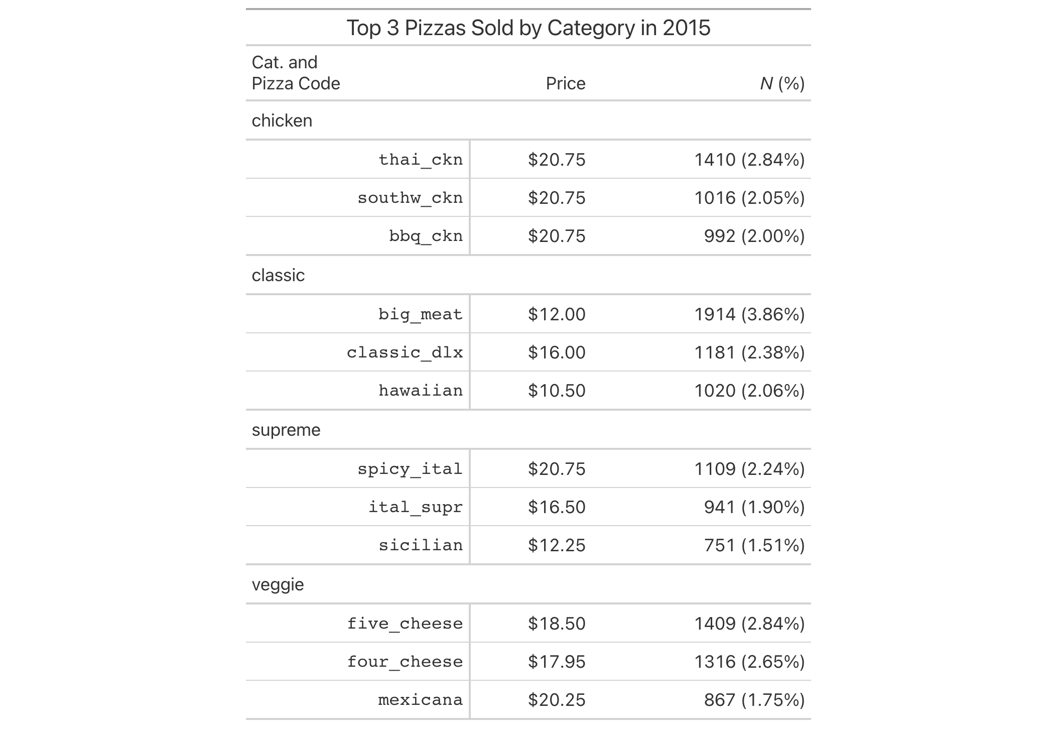
Function ID
5-17
Function Introduced
v0.3.0 (May 12, 2021)
See Also
Other column modification functions:
cols_add(),
cols_align(),
cols_align_decimal(),
cols_hide(),
cols_label(),
cols_label_with(),
cols_merge(),
cols_merge_range(),
cols_merge_uncert(),
cols_move(),
cols_move_to_end(),
cols_move_to_start(),
cols_nanoplot(),
cols_unhide(),
cols_units(),
cols_width()
Merge two columns to a value range column
Description
cols_merge_range() is a specialized variant of cols_merge(). It operates
by taking a two columns that constitute a range of values (col_begin and
col_end) and merges them into a single column. What results is a column
containing both values separated by an em dash. The column specified in
col_end is dropped from the output table.
Usage
cols_merge_range( data, col_begin, col_end, rows = everything(), autohide = TRUE, sep = NULL, locale = NULL )cols_merge_range( data, col_begin, col_end, rows = everything(), autohide = TRUE, sep = NULL, locale = NULL )
Arguments
data |
The gt table or gt group data object
This is the gt table object that is commonly created through use of the
OR
This is the gt group object that is commonly created through use of the
|
col_begin |
Column to target for beginning of range
The column that contains values for the start of the range. While select
helper functions such as |
col_end |
Column to target for end of range
The column that contains values for the end of the range. While select
helper functions such as |
rows |
Rows to target
In conjunction with |
autohide |
Automatic hiding of the
An option to automatically hide the column specified as
|
sep |
Separator text for ranges
The separator text that indicates the values are ranged. If a |
locale |
Locale identifier
An optional locale identifier that can be used for applying a |
Value
An object of class gt_tbl.
Comparison with other column-merging functions
This function could be somewhat replicated using cols_merge(), however,
cols_merge_range() employs the following specialized operations for NA
handling:
-
NAs incol_begin(but notcol_end) result in a display of only -
NAs incol_end(but notcol_begin) result in a display of only thecol_beginvalues only for the merged column (this is the converse of the previous) -
NAs both incol_beginandcol_endresult in missing values for the merged column
Any resulting NA values in the col_begin column following the merge
operation can be easily formatted using sub_missing(). Separate calls of
sub_missing() can be used for the col_begin and col_end columns for
finer control of the replacement values.
This function is part of a set of four column-merging functions. The other
three are the general cols_merge() function and the specialized
cols_merge_uncert() and cols_merge_n_pct() functions. These functions
operate similarly, where the non-target columns can be optionally hidden from
the output table through the hide_columns or autohide options.
Examples
Let's use a subset of the gtcars dataset to create a gt table,
keeping only the model, mpg_c, and mpg_h columns. Merge the "mpg*"
columns together as a single range column (which is labeled as MPG, in
italics) using the cols_merge_range() function. After the merging process,
the column label for the mpg_c column is updated with cols_label() to
better describe the content.
gtcars |>
  dplyr::select(model, starts_with("mpg")) |>
  dplyr::slice(1:8) |>
  gt() |>
  cols_merge_range(
    col_begin = mpg_c,
    col_end = mpg_h
  ) |>
  cols_label(mpg_c = md("*MPG*"))

Function ID
5-16
Function Introduced
v0.2.0.5 (March 31, 2020)
See Also
Other column modification functions:
cols_add(),
cols_align(),
cols_align_decimal(),
cols_hide(),
cols_label(),
cols_label_with(),
cols_merge(),
cols_merge_n_pct(),
cols_merge_uncert(),
cols_move(),
cols_move_to_end(),
cols_move_to_start(),
cols_nanoplot(),
cols_unhide(),
cols_units(),
cols_width()
Merge columns to a value-with-uncertainty column
Description
cols_merge_uncert() is a specialized variant of cols_merge(). It takes as
input a base value column (col_val) and either: (1) a single uncertainty
column, or (2) two columns representing lower and upper uncertainty bounds.
These columns will be essentially merged in a single column (that of
col_val). What results is a column with values and associated
uncertainties, and any columns specified in col_uncert are hidden from
appearing the output table.
Usage
cols_merge_uncert( data, col_val, col_uncert, rows = everything(), sep = " +/- ", autohide = TRUE )cols_merge_uncert( data, col_val, col_uncert, rows = everything(), sep = " +/- ", autohide = TRUE )
Arguments
data |
The gt table or gt group data object
This is the gt table object that is commonly created through use of the
OR
This is the gt group object that is commonly created through use of the
|
col_val |
Column to target for base values
The column that contains values for the start of the range. While select
helper functions such as |
col_uncert |
Column or columns to target for uncertainty values
The most common case involves supplying a single column with uncertainties;
these values will be combined with those in |
rows |
Rows to target
In conjunction with |
sep |
Separator text for uncertainties
The separator text that contains the uncertainty mark for a single
uncertainty value. The default value of |
autohide |
Automatic hiding of the
An option to automatically hide any columns specified in |
Value
An object of class gt_tbl.
Comparison with other column-merging functions
This function could be somewhat replicated using cols_merge() in the case
where a single column is supplied for col_uncert, however,
cols_merge_uncert() employs the following specialized semantics for NA
handling:
-
NAs incol_valresult in missing values for the merged column (e.g.,NA+0.1=NA) -
NAs incol_uncert(but notcol_val) result in base values only for the merged column (e.g.,12.0+NA=12.0) -
NAs bothcol_valandcol_uncertresult in missing values for the merged column (e.g.,NA+NA=NA)
Any resulting NA values in the col_val column following the merge
operation can be easily formatted using sub_missing().
This function is part of a set of four column-merging functions. The other
three are the general cols_merge() function and the specialized
cols_merge_range() and cols_merge_n_pct() functions. These functions
operate similarly, where the non-target columns can be optionally hidden from
the output table through the hide_columns or autohide options.
Examples
Let's use the exibble dataset to create a simple, two-column gt table
(keeping only the num and currency columns). We'll format the num
column with the fmt_number() function. Next we merge the currency and
num columns into the currency column; this will contain a base value and
an uncertainty and it's all done using the cols_merge_uncert() function.
After the merging process, the column label for the currency column is
updated with cols_label() to better describe the content.
exibble |>
  dplyr::select(num, currency) |>
  dplyr::slice(1:7) |>
  gt() |>
  fmt_number(
    columns = num,
    decimals = 3,
    use_seps = FALSE
  ) |>
  cols_merge_uncert(
    col_val = currency,
    col_uncert = num
  ) |>
  cols_label(currency = "value + uncert.")

Function ID
5-15
Function Introduced
v0.2.0.5 (March 31, 2020)
See Also
Other column modification functions:
cols_add(),
cols_align(),
cols_align_decimal(),
cols_hide(),
cols_label(),
cols_label_with(),
cols_merge(),
cols_merge_n_pct(),
cols_merge_range(),
cols_move(),
cols_move_to_end(),
cols_move_to_start(),
cols_nanoplot(),
cols_unhide(),
cols_units(),
cols_width()
Move one or more columns
Description
On those occasions where you need to move columns this way or that way, we
can make use of the cols_move() function. While it's true that the movement
of columns can be done upstream of gt, it is much easier and less error
prone to use the function provided here. The movement procedure here takes
one or more specified columns (in the columns argument) and places them to
the right of a different column (the after argument). The ordering of the
columns to be moved is preserved, as is the ordering of all other columns
in the table.
Usage
cols_move(data, columns, after)cols_move(data, columns, after)
Arguments
data |
The gt table or gt group data object
This is the gt table object that is commonly created through use of the
OR
This is the gt group object that is commonly created through use of the
|
columns |
Columns to target
The columns for which the moving operations should be applied. Can either
be a series of column names provided in |
after |
Column used as anchor
The column used to anchor the insertion of the moved columns. All of the
moved columns will be placed to the right of this column. While select
helper functions such as |
Details
The columns supplied in columns must all exist in the table and none of
them can be in the after argument. The after column must also exist and
only one column should be provided here. If you need to place one or more
columns at the beginning of the column series, the cols_move_to_start()
function should be used. Similarly, if those columns to move should be placed
at the end of the column series then use cols_move_to_end().
Value
An object of class gt_tbl.
Examples
Use the countrypops dataset to create a gt table. We'll choose to
position the population column after the country_name column by using the
cols_move() function.
countrypops |>
  dplyr::select(-contains("code")) |>
  dplyr::filter(
    country_name == "Japan",
    year %in% 2012:2021
  ) |>
  gt() |>
  cols_move(
    columns = population,
    after = country_name
  ) |>
  fmt_integer(columns = population)

Function ID
5-9
Function Introduced
v0.2.0.5 (March 31, 2020)
See Also
Other column modification functions:
cols_add(),
cols_align(),
cols_align_decimal(),
cols_hide(),
cols_label(),
cols_label_with(),
cols_merge(),
cols_merge_n_pct(),
cols_merge_range(),
cols_merge_uncert(),
cols_move_to_end(),
cols_move_to_start(),
cols_nanoplot(),
cols_unhide(),
cols_units(),
cols_width()
Move one or more columns to the end
Description
It's possible to move a set of columns to the end of the column series, we
only need to specify which columns are to be moved. While this can be done
upstream of gt, this function makes to process much easier and it's less
error prone. The ordering of the columns that are moved to the end is
preserved (same with the ordering of all other columns in the table).
Usage
cols_move_to_end(data, columns)cols_move_to_end(data, columns)
Arguments
data |
The gt table or gt group data object
This is the gt table object that is commonly created through use of the
OR
This is the gt group object that is commonly created through use of the
|
columns |
Columns to target
The columns for which the moving operations should be applied. Can either
be a series of column names provided in |
Details
The columns supplied in columns must all exist in the table. If you need to
place one or columns at the start of the column series, cols_move_to_start()
should be used. More control is offered with cols_move(), where columns
could be placed after a specific column.
Value
An object of class gt_tbl.
Examples
For this example, we'll use a portion of the countrypops dataset to
create a simple gt table. Let's move the year column, which is the
middle column, to the end of the column series with cols_move_to_end().
countrypops |>
  dplyr::select(-contains("code")) |>
  dplyr::filter(
    country_name == "Benin",
    year %in% 2017:2021
  ) |>
  gt() |>
  cols_move_to_end(columns = year)

We can also move multiple columns at a time. With the same
countrypops-based table, let's move both the year and country_name
columns to the end of the column series.
countrypops |>
  dplyr::select(-contains("code")) |>
  dplyr::filter(
    country_name == "Benin",
    year %in% 2017:2021
  ) |>
  gt() |>
  cols_move_to_end(columns = c(year, country_name))

Function ID
5-11
Function Introduced
v0.2.0.5 (March 31, 2020)
See Also
Other column modification functions:
cols_add(),
cols_align(),
cols_align_decimal(),
cols_hide(),
cols_label(),
cols_label_with(),
cols_merge(),
cols_merge_n_pct(),
cols_merge_range(),
cols_merge_uncert(),
cols_move(),
cols_move_to_start(),
cols_nanoplot(),
cols_unhide(),
cols_units(),
cols_width()
Move one or more columns to the start
Description
We can easily move set of columns to the beginning of the column series and
we only need to specify which columns. It's possible to do this upstream of
gt, however, it is easier with this function and it presents less
possibility for error. The ordering of the columns that are moved to the
start is preserved (same with the ordering of all other columns in the
table).
Usage
cols_move_to_start(data, columns)cols_move_to_start(data, columns)
Arguments
data |
The gt table or gt group data object
This is the gt table object that is commonly created through use of the
OR
This is the gt group object that is commonly created through use of the
|
columns |
Columns to target
The columns for which the moving operations should be applied. Can either
be a series of column names provided in |
Details
The columns supplied in columns must all exist in the table. If you need to
place one or columns at the end of the column series, cols_move_to_end()
should be used. More control is offered with cols_move(), where columns
could be placed after a specific column.
Value
An object of class gt_tbl.
Examples
For this example, we'll use a portion of the countrypops dataset to
create a simple gt table. Let's move the year column, which is the
middle column, to the start of the column series with cols_move_to_start().
countrypops |>
  dplyr::select(-contains("code")) |>
  dplyr::filter(
    country_name == "Fiji",
    year %in% 2017:2021
  ) |>
  gt() |>
  cols_move_to_start(columns = year)

We can also move multiple columns at a time. With the same
countrypops-based table, let's move both the year and population
columns to the start of the column series.
countrypops |>
  dplyr::select(-contains("code")) |>
  dplyr::filter(
    country_name == "Fiji",
    year %in% 2017:2021
  ) |>
  gt() |>
  cols_move_to_start(columns = c(year, population))

Function ID
5-10
Function Introduced
v0.2.0.5 (March 31, 2020)
See Also
Other column modification functions:
cols_add(),
cols_align(),
cols_align_decimal(),
cols_hide(),
cols_label(),
cols_label_with(),
cols_merge(),
cols_merge_n_pct(),
cols_merge_range(),
cols_merge_uncert(),
cols_move(),
cols_move_to_end(),
cols_nanoplot(),
cols_unhide(),
cols_units(),
cols_width()
Add a new column of nanoplots, taking input data from selected columns
Description
Nanoplots are tiny plots you can use in your gt table. They are simple by
design, mainly because there isn't a lot of space to work with. With that
simplicity, however, you do get a set of very succinct data visualizations
that adapt nicely to the amount of data you feed into them. With
cols_nanoplot() you take data from one or more columns as the basic inputs
for the nanoplots and generate a new column containing the plots. The
nanoplots are robust against missing values, and multiple strategies are
available for handling missingness.
Nanoplots try to show individual data with reasonably good visibility.
Interactivity is included as a basic feature so one can hover over the data
points and vertical guides will display the value ascribed to each data
point. Because gt knows all about numeric formatting, values will be
compactly formatted so as to not take up valuable real estate. If you need to
create a nanoplot based on monetary values, that can be handled by providing
the currency code to the nanoplot_options() helper (then hook that up to
the options argument). A guide on the left-hand side of the plot area will
appear on hover and display the minimal and maximal y values.
There are three types of nanoplots available: "line", "bar", "boxplot".
A line plot shows individual data points and has smooth connecting lines
between them to allow for easier scanning of values. You can opt for
straight-line connections between data points, or, no connections at all
(it's up to you). You can even eschew the data points and just have a simple
line. Regardless of how you mix and match difference plot layers, the plot
area focuses on the domain of the data points with the goal of showing you
the overall trend of the data. The data you feed into a line plot can consist
of a single vector of values (resulting in equally-spaced y values), or,
you can supply two vectors representative of x and y.
A bar plot is built a little bit differently. The focus is on evenly-spaced bars (requiring a single vector of values) that project from a zero line, clearly showing the difference between positive and negative values. By default, any type of nanoplot will have basic interactivity. One can hover over the data points and vertical guides will display values ascribed to each. A guide on the left-hand side of the plot area will display the minimal and maximal y values on hover.
Every box plot will take the collection of values for a row and construct the plot horizontally. This is essentially a standard box-and-whisker diagram where outliers are automatically displayed outside the left and right fences.
While basic customization options are present in the cols_nanoplot(), many
more opportunities for customizing nanoplots on a more granular level are
possible with the nanoplot_options() helper function. That function should
be invoked at the options argument of cols_nanoplot(). Through that
helper, layers of the nanoplots can be selectively removed and the aesthetics
of the remaining plot components can be modified.
Usage
cols_nanoplot( data, columns, rows = everything(), plot_type = c("line", "bar", "boxplot"), plot_height = "2em", missing_vals = c("gap", "marker", "zero", "remove"), autoscale = FALSE, autohide = TRUE, columns_x_vals = NULL, reference_line = NULL, reference_area = NULL, expand_x = NULL, expand_y = NULL, new_col_name = NULL, new_col_label = NULL, before = NULL, after = NULL, options = NULL )cols_nanoplot( data, columns, rows = everything(), plot_type = c("line", "bar", "boxplot"), plot_height = "2em", missing_vals = c("gap", "marker", "zero", "remove"), autoscale = FALSE, autohide = TRUE, columns_x_vals = NULL, reference_line = NULL, reference_area = NULL, expand_x = NULL, expand_y = NULL, new_col_name = NULL, new_col_label = NULL, before = NULL, after = NULL, options = NULL )
Arguments
data |
The gt table or gt group data object
This is the gt table object that is commonly created through use of the
OR
This is the gt group object that is commonly created through use of the
|
columns |
Columns from which to get data for the dependent variable
The columns which contain the numeric data to be plotted as nanoplots. Can
either be a series of column names provided in |
rows |
Rows that should contain nanoplots
With |
plot_type |
The type of nanoplot to display
Nanoplots can either take the form of a line plot (using |
plot_height |
The height of the nanoplots
The height of the nanoplots. The default here is a sensible value of
|
missing_vals |
Treatment of missing values
If missing values are encountered within the input data, there are three
strategies available for their handling: (1) |
autoscale |
Automatically set x- and y-axis scale limits based on data
Using |
autohide |
Automatically hide the
An option to automatically hide any columns specified in |
columns_x_vals |
Columns containing values for the optional x variable
We can optionally obtain data for the independent variable (i.e., the
x-axis data) if specifying columns in |
reference_line |
Add a reference line
A reference line requires a single input to define the line. It could be a
static numeric value, applied to all nanoplots generated. Or, the input can
be one of the following for generating the line from the underlying data:
(1) |
reference_area |
Add a reference area
A reference area requires two inputs to define bottom and top boundaries
for a rectangular area. The types of values supplied are the same as those
expected for |
expand_x, expand_y
|
Expand plot scale in the x and y directions
Should you need to have plots expand in the x or y direction, provide
one or more values to |
new_col_name |
Column name for the new column containing the plots
A single column name in quotation marks. Values will be extracted from this
column and provided to compatible arguments. If not provided the new column
name will be |
new_col_label |
Column label for the new column containing the plots
A single column label. If not supplied then the column label will inherit
from |
before, after
|
Column used as anchor
A single column-resolving expression or column index can be given to either
|
options |
Set options for the nanoplots
By using the |
Value
An object of class gt_tbl.
Targeting cells with columns and rows
Targeting of values to insert into the nanoplots is done through columns
and additionally by rows (if nothing is provided for rows then entire
columns are selected). Aside from declaring column names in c() (with bare
column names or names in quotes) we can use also
tidyselect-style expressions. This can be as basic as supplying a select
helper like starts_with(), or, providing a more complex incantation like
where(~ is.numeric(.x) & max(.x, na.rm = TRUE) > 1E6)
which targets numeric columns that have a maximum value greater than
1,000,000 (excluding any NAs from consideration).
Once the columns are targeted, we may also target the rows within those
columns. This can be done in a variety of ways. If a stub is present, then we
potentially have row identifiers. Those can be used much like column names in
the columns-targeting scenario. We can use simpler tidyselect-style
expressions (the select helpers should work well here) and we can use quoted
row identifiers in c(). It's also possible to use row indices (e.g.,
c(3, 5, 6)) though these index values must correspond to the row numbers of
the input data (the indices won't necessarily match those of rearranged rows
if row groups are present). One more type of expression is possible, an
expression that takes column values (can involve any of the available columns
in the table) and returns a logical vector.
How to supply data for nanoplots
The input data for nanoplots naturally needs to be numeric and there are two
major ways to formulate that data: (1) from single values across many
columns, and (2) using text-based value streams. It's pretty easy to
rationalize the first, and we may already have wide data in the input data
frame anyway (take a look at the illness and towny datasets for
examples of this). There's one data value per column so the key thing here is
to reference the columns in the correct order. With a select helper, good
column naming, and the columns being in the intended order, this is a snap.
The second option is to use text-based value streams. Sometimes you simply
don't want or don't need multiple columns and so a single column with all of
the data might be more practical. To make this work, you'd need to have a set
of numerical values separated by some sort of delimiter (could be a comma, a
space, a semicolon, you get the idea). Here's an example with three numbers,
written three ways: "3.6 -2.44 1.98", "3.6, -2.44, 1.98", and
"3.6;-2.44;1.98". You can include NA values, not a problem, and here's an
example of that: "6.232 NA 3.7 0.93". Another form of value stream involves
using datetimes in the ISO 8601 form of YYYY-MM-DD HH:MM:SS. These will
be internally converted to numeric values (seconds elapsed since
"1970-01-01 00:00:00"). An example of a datetime-based value stream is:
"2012-06-12 08:24:13, 2012-06-12 10:37:08, 2012-06-12 14:03:24".
Value streams can be pretty big if you want them to be, and you don't have to
deal with containing individual values across multiple columns. For the case
where you need to provide two sets of values (x and y, for line plots
with columns and columns_x_vals), have two equivalently sized value
streams in two columns. Value streams can also be concatenated together by
referencing columns having their own separate value streams.
Reference line and reference area
Neither a horizontal reference line nor a reference area is present in
the default view but these can be added by providing valid input values in
the reference_line and reference_area arguments. A reference line can
be either be a static numeric value (supply any number to reference_line),
or it can be a keyword that computes the reference line y value using the
data values for each nanoplot. The following keywords can be used:
-
"mean": The mean of the data values -
"median": Median of data values -
"min": Minimum value in set of data values -
"max": The maximum value -
"q1": The first, or lower, quartile of the data values -
"q3": The third quartile, otherwise known as the upper quartile -
"first": The first data value -
"last": The last data value
The reference area accepts two inputs, and this can be two of the above keywords, a keyword and a static numeric value, or two numeric values.
Examples
Let's make some nanoplots with the illness dataset. The columns beginning
with 'day' all contain ordered measurement values, comprising seven
individual daily results. Using cols_nanoplot() we create a new column to
hold the nanoplots (with new_col_name = "nanoplots"), referencing the
columns containing the data (with columns = starts_with("day")). It's also
possible to define a column label here using the new_col_label argument.
illness |>
  dplyr::slice_head(n = 10) |>
  gt(rowname_col = "test") |>
  tab_header("Partial summary of daily tests performed on YF patient") |>
  tab_stubhead(label = md("**Test**")) |>
  cols_hide(columns = starts_with("norm")) |>
  fmt_units(columns = units) |>
  cols_nanoplot(
    columns = starts_with("day"),
    new_col_name = "nanoplots",
    new_col_label = md("*Progression*")
  ) |>
  cols_align(align = "center", columns = nanoplots) |>
  cols_merge(columns = c(test, units), pattern = "{1} ({2})") |>
  tab_footnote(
    footnote = "Measurements from Day 3 through to Day 8.",
    locations = cells_column_labels(columns = nanoplots)
  )

The previous table showed us some line-based nanoplots. We can also make very
small bar plots with cols_nanoplot(). Let's take the pizzaplace dataset
and make a small summary table showing daily pizza sales by type (there are
four types). This will be limited to the first ten days of pizza sales in
2015, so, there will be ten rows in total. We can use plot_type = "bar" to
make bar plots from the daily sales counts in the chicken, classic,
supreme, and veggie columns. Because we know there will always be four
bars (one for each type of pizza) we can be a little creative and apply
colors to each of the bars through use of the data_bar_fill_color argument
in nanoplot_options().
pizzaplace |>
  dplyr::count(type, date) |>
  tidyr::pivot_wider(names_from = type, values_from = n) |>
  dplyr::slice_head(n = 10) |>
  gt(rowname_col = "date") |>
  tab_header(
    title = md("First Ten Days of Pizza Sales in 2015")
  ) |>
  cols_nanoplot(
    columns = c(chicken, classic, supreme, veggie),
    plot_type = "bar",
    autohide = FALSE,
    new_col_name = "pizzas_sold",
    new_col_label = "Sales by Type",
    options = nanoplot_options(
      show_data_line = FALSE,
      show_data_area = FALSE,
      data_bar_stroke_color = "transparent",
      data_bar_fill_color = c("brown", "gold", "purple", "green")
    )
  ) |>
  cols_width(pizzas_sold ~ px(150)) |>
  cols_align(columns = -date, align = "center") |>
  fmt_date(columns = date, date_style = "yMMMEd") |>
  opt_all_caps()

Now we'll make another table that contains two columns of nanoplots. Starting
from the towny dataset, we first reduce it down to a subset of columns
and rows. All of the columns related to either population or density will be
used as input data for the two nanoplots. Both nanoplots will use a reference
line that is generated from the median of the input data. And by naming the
new nanoplot-laden columns in a similar manner as the input data columns, we
can take advantage of select helpers (e.g., when using tab_spanner()). Many
of the input data columns are now redundant because of the plots, so we'll
elect to hide most of those with cols_hide().
towny |>
  dplyr::select(name, starts_with("population"), starts_with("density")) |>
  dplyr::filter(population_2021 > 200000) |>
  dplyr::arrange(desc(population_2021)) |>
  gt() |>
  fmt_integer(columns = starts_with("population")) |>
  fmt_number(columns = starts_with("density"), decimals = 1) |>
  cols_nanoplot(
    columns = starts_with("population"),
    reference_line = "median",
    autohide = FALSE,
    new_col_name = "population_plot",
    new_col_label = md("*Change*")
  ) |>
  cols_nanoplot(
    columns = starts_with("density"),
    plot_type = "bar",
    autohide = FALSE,
    new_col_name = "density_plot",
    new_col_label = md("*Change*")
  ) |>
  cols_hide(columns = matches("2001|2006|2011|2016")) |>
  tab_spanner(
    label = "Population",
    columns = starts_with("population")
  ) |>
  tab_spanner(
    label = "Density ({{*persons* km^-2}})",
    columns = starts_with("density")
  ) |>
  cols_label_with(
    columns = -matches("plot"),
    fn = function(x) gsub("[^0-9]+", "", x)
  ) |>
  cols_align(align = "center", columns = matches("plot")) |>
  cols_width(
    name ~ px(140),
    everything() ~ px(100)
  ) |>
  opt_horizontal_padding(scale = 2)

The sza dataset can, with just some use of dplyr and tidyr, give
us a wide table full of nanoplottable values. We'll transform the solar
zenith angles to solar altitude angles and create a column of nanoplots using
the newly calculated values. There are a few NA values during periods where
the sun hasn't risen (usually before 06:30 in the winter months) and those
values will be replaced with 0 using missing_vals = "zero". We'll also
elect to create bar plots using the plot_type = "bar" option. The height of
the plots will be bumped up to "2.5em" from the default of "2em".
Finally, we will use nanoplot_options() to modify the coloring of the data
bars.
sza |>
  dplyr::filter(latitude == 20 & tst <= "1200") |>
  dplyr::select(-latitude) |>
  dplyr::filter(!is.na(sza)) |>
  dplyr::mutate(saa = 90 - sza) |>
  dplyr::select(-sza) |>
  tidyr::pivot_wider(
    names_from = tst,
    values_from = saa,
    names_sort = TRUE
  ) |>
  gt(rowname_col = "month") |>
  tab_header(
    title = "Solar Altitude Angles",
    subtitle = "Average values every half hour from 05:30 to 12:00"
  ) |>
  cols_nanoplot(
    columns = matches("0"),
    plot_type = "bar",
    missing_vals = "zero",
    new_col_name = "saa",
    plot_height = "2.5em",
    options = nanoplot_options(
      data_bar_stroke_color = "GoldenRod",
      data_bar_fill_color = "DarkOrange"
    )
  ) |>
  tab_options(
    table.width = px(400),
    column_labels.hidden = TRUE
  ) |>
  cols_align(
    align = "center",
    columns = everything()
  ) |>
  tab_source_note(
    source_note = "The solar altitude angle is the complement to
    the solar zenith angle. TMYK."
  )

You can use number and time streams as data for nanoplots. Let's demonstrate
how we can make use of them with some creative transformation of the
pizzaplace dataset. A value stream is really a string with delimited
numeric values, like this: "7.24,84.2,14". A value stream can also contain
dates and/or datetimes, and here's an example of that:
"2020-06-02 13:05:13,2020-06-02 14:24:05,2020-06-02 18:51:37". Having data
in this form can often be more convenient since different nanoplots might
have varying amounts of data (and holding different amounts of data in a
fixed number of columns is cumbersome). There are date and time columns
in this dataset and we'll use that to get x values denoting high-resolution
time instants: the second of the day that a pizza was sold (this is true
pizza analytics). We also have the sell price for a pizza, and that'll serve
as the y values. The pizzas belong to four different groups (in the type
column) and we'll group by that and create value streams with
paste(..., collapse = ",") inside the dplyr::summarize() call. With two
value streams in each row (having the same number of values) we can now make
a gt table with nanoplots.
pizzaplace |>
  dplyr::filter(date == "2015-01-01") |>
  dplyr::mutate(date_time = paste(date, time)) |>
  dplyr::select(type, date_time, price) |>
  dplyr::group_by(type) |>
  dplyr::summarize(
    date_time = paste(date_time, collapse = ","),
    sold = paste(price, collapse = ",")
  ) |>
  gt(rowname_col = "type") |>
  tab_header(
    title = md("Pizzas sold on **January 1, 2015**"),
    subtitle = "Between the opening hours of 11:30 to 22:30"
  ) |>
  cols_nanoplot(
    columns = sold,
    columns_x_vals = date_time,
    expand_x = c("2015-01-01 11:30", "2015-01-01 22:30"),
    reference_line = "median",
    new_col_name = "pizzas_sold",
    new_col_label = "Pizzas Sold",
    options = nanoplot_options(
      show_data_line = FALSE,
      show_data_area = FALSE,
      currency = "USD"
    )
  ) |>
  cols_width(pizzas_sold ~ px(200)) |>
  cols_align(columns = pizzas_sold, align = "center") |>
  opt_all_caps()

Notice that the columns containing the value streams are hid due to the
default argument autohide = TRUE because, while useful, they don't need to
be displayed to anybody viewing a table. Since we have a lot of data points
and a connecting line is not as valuable here, we also set
show_data_line = FALSE in nanoplot_options(). It's more interesting to
see the clusters of the differently priced pizzas over the entire day.
Specifying a currency in nanoplot_options() is a nice touch since the y
values are sale prices in U.S. Dollars (hovering over data points gives
correctly formatted values). Finally, having a reference line based on the
median gives pretty useful information. Seems like customers preferred
getting the "chicken"-type pizzas in large size!
Using the gibraltar dataset, let's make a series of nanoplots across the
meteorological parameters of temperature, humidity, and wind speed. We'll
want to customize the appearance of the plots across three columns and we
can make this somewhat simpler by assigning a common set of options through
nanoplot_options(). In this table we want to make comparisons across
nanoplots in a particular column easier, so, we'll set autoscale = TRUE so
that there is a common y-axis scale for each of the parameters (based on the
extents of the data).
nanoplot_options_list <-
  nanoplot_options(
    data_point_radius = px(4),
    data_point_stroke_width = px(2),
    data_point_stroke_color = "black",
    data_point_fill_color = "white",
    data_line_stroke_width = px(4),
    data_line_stroke_color = "gray",
    show_data_line = TRUE,
    show_data_points = TRUE,
    show_data_area = FALSE,
  )

gibraltar |>
  dplyr::filter(date <= "2023-05-14") |>
  dplyr::mutate(time = as.numeric(hms::as_hms(paste0(time, ":00")))) |>
  dplyr::mutate(humidity = humidity * 100) |>
  dplyr::select(date, time, temp, humidity, wind_speed) |>
  dplyr::group_by(date) |>
  dplyr::summarize(
    time = paste(time, collapse = ","),
    temp = paste(temp, collapse = ","),
    humidity = paste(humidity, collapse = ","),
    wind_speed = paste(wind_speed, collapse = ","),
  ) |>
  dplyr::mutate(is_satsun = lubridate::wday(date) %in% c(1, 7)) |>
  gt(rowname_col = "date") |>
  tab_header(
    title = "Meteorological Summary of Gibraltar Station",
    subtitle = "Data taken from May 1-14, 2023."
  ) |>
  fmt_date(columns = stub(), date_style = "wd_m_day_year") |>
  cols_nanoplot(
    columns = temp,
    columns_x_vals = time,
    expand_x = c(0, 86400),
    autoscale = TRUE,
    new_col_name = "temperature_nano",
    new_col_label = "Temperature",
    options = nanoplot_options_list
  ) |>
  cols_nanoplot(
    columns = humidity,
    columns_x_vals = time,
    expand_x = c(0, 86400),
    autoscale = TRUE,
    new_col_name = "humidity_nano",
    new_col_label = "Humidity",
    options = nanoplot_options_list
  ) |>
  cols_nanoplot(
    columns = wind_speed,
    columns_x_vals = time,
    expand_x = c(0, 86400),
    autoscale = TRUE,
    new_col_name = "wind_speed_nano",
    new_col_label = "Wind Speed",
    options = nanoplot_options_list
  ) |>
  cols_units(
    temperature_nano = ":degree:C",
    humidity_nano = "% (RH)",
    wind_speed_nano = "m s^-1"
  ) |>
  cols_hide(columns = is_satsun) |>
  tab_style_body(
    style = cell_fill(color = "#E5FEFE"),
    values = TRUE,
    targets = "row",
    extents = c("body", "stub")
  ) |>
  tab_style(
    style = cell_text(align = "center"),
    locations = cells_column_labels()
  )

Box plots can be generated, and we just need to use plot_type = "boxplot"
to make that type of nanoplot. Using a small portion of the pizzaplace
dataset, we will create a simple table that displays a box plot of pizza
sales for a selection of days. By converting the string-time 24-hour-clock
time values to the number of seconds elapsed in a day, we get continuous
values that can be incorporated into each box plot. And, by supplying a
function to the y_val_fmt_fn argument within nanoplot_options(), we can
transform the integer seconds values back to clock times for display on
hover.
pizzaplace |>
  dplyr::filter(date <= "2015-01-14") |>
  dplyr::mutate(time = as.numeric(hms::as_hms(time))) |>
  dplyr::summarize(time = paste(time, collapse = ","), .by = date) |>
  dplyr::mutate(is_weekend = lubridate::wday(date) %in% 6:7) |>
  gt() |>
  tab_header(title = "Pizza Sales in Early January 2015") |>
  fmt_date(columns = date, date_style = 2) |>
  cols_nanoplot(
    columns = time,
    plot_type = "boxplot",
    options = nanoplot_options(y_val_fmt_fn = function(x) hms::as_hms(x))
  ) |>
  cols_hide(columns = is_weekend) |>
  cols_width(everything() ~ px(250)) |>
  cols_align(align = "center", columns = nanoplots) |>
  cols_align(align = "left", columns = date) |>
  tab_style(
    style = cell_borders(
      sides = "left", color = "gray"),
    locations = cells_body(columns = nanoplots)
  ) |>
  tab_style_body(
    style = cell_fill(color = "#E5FEFE"),
    values = TRUE,
    targets = "row"
  ) |>
  tab_options(column_labels.hidden = TRUE)

Function ID
5-8
Function Introduced
v0.10.0 (October 7, 2023)
See Also
Other column modification functions:
cols_add(),
cols_align(),
cols_align_decimal(),
cols_hide(),
cols_label(),
cols_label_with(),
cols_merge(),
cols_merge_n_pct(),
cols_merge_range(),
cols_merge_uncert(),
cols_move(),
cols_move_to_end(),
cols_move_to_start(),
cols_unhide(),
cols_units(),
cols_width()
Unhide one or more columns
Description
cols_unhide() allows us to take one or more hidden columns (usually done
via cols_hide()) and make them visible in the final output table. This may
be important in cases where the user obtains a gt_tbl object with hidden
columns and there is motivation to reveal one or more of those.
Usage
cols_unhide(data, columns)cols_unhide(data, columns)
Arguments
data |
The gt table or gt group data object
This is the gt table object that is commonly created through use of the
OR
This is the gt group object that is commonly created through use of the
|
columns |
Columns to target
The columns to unhide in the output display table. Can either be a series
of column names provided in |
Details
The hiding and unhiding of columns is internally a rendering directive, so,
all columns that are 'hidden' are still accessible and useful in any
expression provided to a rows argument. The cols_unhide() function
quietly changes the visible state of a column (much like the cols_hide()
function) and doesn't yield warnings or messages when changing the state of
already-visible columns.
Value
An object of class gt_tbl.
Examples
Let's use a small portion of the countrypops dataset to create a gt
table. We'll hide the country_code_2 and country_code_3 columns with
cols_hide().
tab_1 <-
  countrypops |>
  dplyr::filter(
    country_name == "Singapore",
    year %in% 2017:2021
  ) |>
  gt() |>
  cols_hide(columns = c(country_code_2, country_code_3))

tab_1

If the tab_1 object is provided without the code or source data to
regenerate it, and, the user wants to reveal otherwise hidden columns then
cols_unhide() becomes useful.
tab_1 |> cols_unhide(columns = country_code_2)

Function ID
5-13
Function Introduced
v0.3.0 (May 12, 2021)
See Also
cols_hide() to perform the inverse operation.
Other column modification functions:
cols_add(),
cols_align(),
cols_align_decimal(),
cols_hide(),
cols_label(),
cols_label_with(),
cols_merge(),
cols_merge_n_pct(),
cols_merge_range(),
cols_merge_uncert(),
cols_move(),
cols_move_to_end(),
cols_move_to_start(),
cols_nanoplot(),
cols_units(),
cols_width()
Define units for one or more columns
Description
Column labels can sometimes contain measurement units, and these might range
from easy to define and typeset (e.g., "m/s") to very difficult. Such
difficulty can arise from the need to include subscripts or superscripts,
non-ASCII symbols, etc. The cols_units() function tries to make this task
easier by letting you apply text pertaining to units to various columns. This
takes advantage of gt's specialized units notation (e.g.,
"J Hz^-1 mol^-1" can be used to generate units for the
molar Planck constant). The notation here provides several conveniences for
defining units, letting you produce the correct formatting no matter what the
table output format might be (i.e., HTML, LaTeX, RTF, etc.). Details
pertaining to the units notation can be found in the section entitled
How to use gt's units notation.
Usage
cols_units(.data, ..., .list = list2(...), .units_pattern = NULL)cols_units(.data, ..., .list = list2(...), .units_pattern = NULL)
Arguments
.data |
The gt table or gt group data object
This is the gt table object that is commonly created through use of the
OR
This is the gt group object that is commonly created through use of the
|
... |
Column units definitions
Expressions for the assignment of column units for the table columns in
|
.list |
Alternative to
Allows for the use of a list as an input alternative to |
.units_pattern |
Pattern to combine column labels and units
An optional pattern to be used for combining column labels with the defined
units. The default pattern is |
Value
An object of class gt_tbl.
How to use gt's units notation
The units notation involves a shorthand of writing units that feels familiar and is fine-tuned for the task at hand. Each unit is treated as a separate entity (parentheses and other symbols included) and the addition of subscript text and exponents is flexible and relatively easy to formulate. This is all best shown with examples:
-
"m/s"and"m / s"both render as"m/s" -
"m s^-1"will appear with the"-1"exponent intact -
"m /s"gives the same result, as"/<unit>"is equivalent to"<unit>^-1" -
"E_h"will render an"E"with the"h"subscript -
"t_i^2.5"provides atwith an"i"subscript and a"2.5"exponent -
"m[_0^2]"will use overstriking to set both scripts vertically -
"g/L %C6H12O6%"uses a chemical formula (enclosed in a pair of"%"characters) as a unit partial, and the formula will render correctly with subscripted numbers -
Common units that are difficult to write using ASCII text may be implicitly converted to the correct characters (e.g., the
"u"in"ug","um","uL", and"umol"will be converted to the Greek mu symbol;"degC"and"degF"will render a degree sign before the temperature unit) -
We can transform shorthand symbol/unit names enclosed in
":"(e.g.,":angstrom:",":ohm:", etc.) into proper symbols -
Greek letters can added by enclosing the letter name in
":"; you can use lowercase letters (e.g.,":beta:",":sigma:", etc.) and uppercase letters too (e.g.,":Alpha:",":Zeta:", etc.) -
The components of a unit (unit name, subscript, and exponent) can be fully or partially italicized/emboldened by surrounding text with
"*"or"**"
Examples
Let's analyze some pizzaplace data with dplyr and then make a gt
table. Here we are separately defining new column labels with cols_label()
and then defining the units (to combine to those labels) through
cols_units(). The default pattern for combination is "{1}, {2}" which
is acceptable here.
pizzaplace |>
  dplyr::mutate(month = lubridate::month(date, label = TRUE, abbr = TRUE)) |>
  dplyr::group_by(month) |>
  dplyr::summarize(
    n_sold = dplyr::n(),
    rev = sum(price)
  ) |>
  dplyr::mutate(chg = (rev - dplyr::lag(rev)) / dplyr::lag(rev)) |>
  dplyr::mutate(month = as.character(month)) |>
  gt(rowname_col = "month") |>
  fmt_integer(columns = n_sold) |>
  fmt_currency(columns = rev, use_subunits = FALSE) |>
  fmt_percent(columns = chg) |>
  sub_missing() |>
  cols_label(
    n_sold = "Number of Pizzas Sold",
    rev = "Revenue Generated",
    chg = "Monthly Changes in Revenue"
  ) |>
  cols_units(
    n_sold = "units month^-1",
    rev = "USD month^-1",
    chg = "% change *m*/*m*"
  ) |>
  cols_width(
    stub() ~ px(40),
    everything() ~ px(200)
  )

The sza dataset has a wealth of information and here we'll generate
a smaller table that contains the average solar zenith angles at noon for
different months and at different northern latitudes. The column labels are
numbers representing the latitudes and it's convenient to apply units
of 'degrees north' to each of them with cols_units(). The extra thing we
wanted to do here was to ensure that the units are placed directly after
the column labels, and we do that with .units_pattern = "{1}{2}". This
append the units ("{2}") right to the column label ("{1}").
sza |>
  dplyr::filter(tst == "1200") |>
  dplyr::select(-tst) |>
  dplyr::arrange(desc(latitude)) |>
  tidyr::pivot_wider(
    names_from = latitude,
    values_from = sza
  ) |>
  gt(rowname_col = "month") |>
  cols_units(
    everything() ~ ":degree:N",
    .units_pattern = "{1}{2}"
  ) |>
  tab_spanner(
    label = "Solar Zenith Angle",
    columns = everything()
  ) |>
  text_transform(
    fn = toupper,
    locations = cells_stub()
  ) |>
  tab_style(
    style = cell_text(align = "right"),
    locations = cells_stub()
  )

Taking a portion of the towny dataset, let's use spanners to describe
what's in the columns and use only measurement units for the column labels.
The columns labels that have to do with population and density information
will be replaced with units defined in cols_units(). We'll use a
.units_pattern value of "{2}", which means that only the units will
be present (the "{1}", representing the column label text, is omitted).
Spanners added through several invocations of tab_spanner() will declare
what the last four columns contain.
towny |>
  dplyr::select(
    name, land_area_km2,
    ends_with("2016"), ends_with("2021")
  ) |>
  dplyr::slice_max(population_2021, n = 10) |>
  gt(rowname_col = "name") |>
  tab_stubhead(label = "City") |>
  fmt_integer() |>
  cols_label(
    land_area_km2 ~ "Area, {{km^2}}",
    starts_with("population") ~ "",
    starts_with("density") ~ ""
  ) |>
  cols_units(
    starts_with("population") ~ "*ppl*",
    starts_with("density") ~ "*ppl* km^-2",
    .units_pattern = "{2}"
  ) |>
  tab_spanner(
    label = "Population",
    columns = starts_with("population"),
    gather = FALSE
  ) |>
  tab_spanner(
    label = "Density",
    columns = starts_with("density"),
    gather = FALSE
  ) |>
  tab_spanner(
    label = "2016",
    columns = ends_with("2016"),
    gather = FALSE
  ) |>
  tab_spanner(
    label = "2021",
    columns = ends_with("2021"),
    gather = FALSE
  ) |>
  tab_style(
    style = cell_text(align = "center"),
    locations = cells_column_labels(
      c(starts_with("population"), starts_with("density"))
    )
  ) |>
  cols_width(everything() ~ px(120)) |>
  opt_horizontal_padding(scale = 3)

Function ID
5-6
Function Introduced
v0.10.0 (October 7, 2023)
See Also
Other column modification functions:
cols_add(),
cols_align(),
cols_align_decimal(),
cols_hide(),
cols_label(),
cols_label_with(),
cols_merge(),
cols_merge_n_pct(),
cols_merge_range(),
cols_merge_uncert(),
cols_move(),
cols_move_to_end(),
cols_move_to_start(),
cols_nanoplot(),
cols_unhide(),
cols_width()
Set the widths of columns
Description
Manual specifications of column widths can be performed using the
cols_width() function. We choose which columns get specific widths. This
can be in units of pixels (easily set by use of the px() helper function),
or, as percentages (where the pct() helper function is useful). Width
assignments are supplied in ... through two-sided formulas, where the
left-hand side defines the target columns and the right-hand side is a single
dimension.
Usage
cols_width(.data, ..., .list = list2(...))cols_width(.data, ..., .list = list2(...))
Arguments
.data |
The gt table or gt group data object
This is the gt table object that is commonly created through use of the
OR
This is the gt group object that is commonly created through use of the
|
... |
Column width assignments
Expressions for the assignment of column widths for the table columns in
|
.list |
Alternative to
Allows for the use of a list as an input alternative to |
Details
Column widths can be set as absolute or relative values (with px and
percentage values). Those columns not specified are treated as having
variable width. The sizing behavior for column widths depends on the
combination of value types, and, whether a table width has been set (which
could, itself, be expressed as an absolute or relative value). Widths for the
table and its container can be individually modified with the table.width
and container.width arguments within tab_options()).
Value
An object of class gt_tbl.
Examples
Use select columns from the exibble dataset to create a gt table. We
can specify the widths of columns with cols_width(). This is done with
named arguments in ..., specifying the exact widths for table columns
(using everything() at the end will capture all remaining columns).
exibble |>
  dplyr::select(
    num, char, date,
    datetime, row
  ) |>
  gt() |>
  cols_width(
    num ~ px(150),
    ends_with("r") ~ px(100),
    starts_with("date") ~ px(200),
    everything() ~ px(60)
  )

Function ID
5-3
Function Introduced
v0.2.0.5 (March 31, 2020)
See Also
Other column modification functions:
cols_add(),
cols_align(),
cols_align_decimal(),
cols_hide(),
cols_label(),
cols_label_with(),
cols_merge(),
cols_merge_n_pct(),
cols_merge_range(),
cols_merge_uncert(),
cols_move(),
cols_move_to_end(),
cols_move_to_start(),
cols_nanoplot(),
cols_unhide(),
cols_units()
The fundamental physical constants
Description
This dataset contains values for over 300 basic fundamental constants in nature. The values originate from the 2018 adjustment which is based on the latest relevant precision measurements and improvements of theoretical calculations. Such work has been carried out under the authority of the Task Group on Fundamental Constants (TGFC) of the Committee on Data of the International Science Council (CODATA). These updated values became available on May 20, 2019. They are published at https://physics.nist.gov/cuu/Constants/index.html, a website of the Fundamental Constants Data Center of the National Institute of Standards and Technology (NIST), Gaithersburg, Maryland, USA.
Usage
constantsconstants
Format
A tibble with 354 rows and 4 variables:
- name
-
The name of the constant.
- value
-
The value of the constant.
- uncert
-
The uncertainty associated with the value. If
NAthen the value is seen as an 'exact' value (e.g., an electron volt has the exact value of 1.602 176 634 e-19 J). - sf_value,sf_uncert
-
The number of significant figures associated with the value and any uncertainty value.
- units
-
The units associated with the constant.
Dataset ID and Badge
DATA-12

Dataset Introduced
v0.10.0 (October 7, 2023)
See Also
Other datasets:
countrypops,
exibble,
films,
gibraltar,
gtcars,
illness,
metro,
nuclides,
peeps,
photolysis,
pizzaplace,
reactions,
rx_addv,
rx_adsl,
sp500,
sza,
towny
Examples
dplyr::glimpse(constants)dplyr::glimpse(constants)
Yearly populations of countries from 1960 to 2024
Description
A dataset that presents yearly, total populations of countries. Total
population is based on counts of all residents regardless of legal status or
citizenship. Country identifiers include the English-language country names,
and the 2- and 3-letter ISO 3166-1 country codes. Each row contains a
population value for a given year (from 1960 to 2024). Any NA values
within population indicate the non-existence of the entity during that
year.
Usage
countrypopscountrypops
Format
A tibble with 13,975 rows and 5 variables:
- country_name
-
The name of the country.
- country_code_2, country_code_3
-
The 2- and 3-letter ISO 3166-1 country codes.
- year
-
The year for the population estimate.
- population
-
The population estimate, midway through the year.
Dataset ID and Badge
DATA-1

Dataset Introduced
v0.2.0.5 (March 31, 2020)
Source
https://data.worldbank.org/indicator/SP.POP.TOTL
See Also
Other datasets:
constants,
exibble,
films,
gibraltar,
gtcars,
illness,
metro,
nuclides,
peeps,
photolysis,
pizzaplace,
reactions,
rx_addv,
rx_adsl,
sp500,
sza,
towny
Supply a custom currency symbol to fmt_currency()
Description
The currency() helper function makes it easy to specify a context-aware
currency symbol to currency argument of fmt_currency(). Since gt can
render tables to several output formats, currency() allows for different
variations of the custom symbol based on the output context (which are
html, latex, rtf, and default). The number of decimal places for
the custom currency defaults to 2, however, a value set for the decimals
argument of fmt_currency() will take precedence.
Usage
currency(..., .list = list2(...))currency(..., .list = list2(...))
Arguments
... |
Currency symbols by output context
One or more named arguments using output contexts as the names and currency symbol text as the values. |
.list |
Alternative to
Allows for the use of a list as an input alternative to |
Details
We can use any combination of html, latex, rtf, and default as named
arguments for the currency text in each of the namesake contexts. The
default value is used as a fallback when there doesn't exist a dedicated
currency text value for a particular output context (e.g., when a table is
rendered as HTML and we use currency(latex = "LTC", default = "ltc"), the
currency symbol will be "ltc". For convenience, if we provide only a single
string without a name, it will be taken as the default (i.e.,
currency("ltc") is equivalent to currency(default = "ltc")). However, if
we were to specify currency strings for multiple output contexts, names are
required each and every context.
Value
A list object of class gt_currency.
Examples
Use the exibble dataset to create a gt table. Within the
fmt_currency() call, we'll format the currency column to have currency
values in guilder (a defunct Dutch currency). We can register this custom
currency with the currency() helper function, supplying the "ƒ" HTML
entity for html outputs and using "f" for any other type of gt
output.
exibble |>
  gt() |>
  fmt_currency(
    columns = currency,
    currency = currency(
      html = "ƒ",
      default = "f"
    ),
    decimals = 2
  )
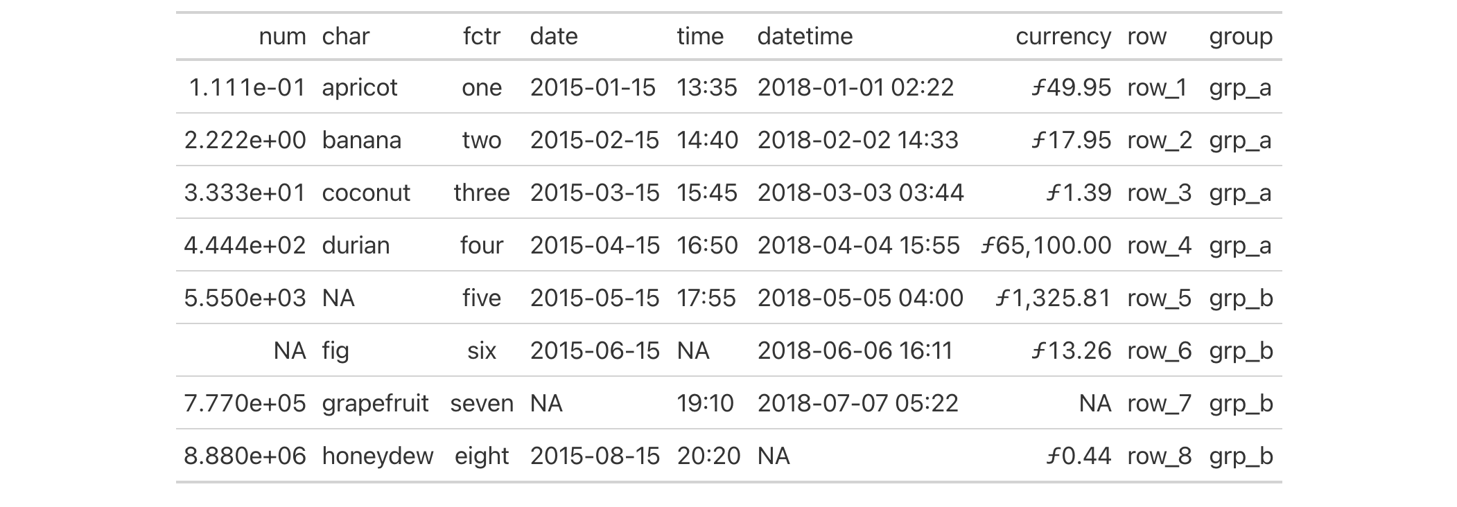
Function ID
8-6
Function Introduced
v0.2.0.5 (March 31, 2020)
See Also
Other helper functions:
adjust_luminance(),
cell_borders(),
cell_fill(),
cell_text(),
default_fonts(),
escape_latex(),
from_column(),
google_font(),
gt_latex_dependencies(),
html(),
latex(),
md(),
nanoplot_options(),
pct(),
px(),
random_id(),
row_group(),
stub(),
system_fonts(),
unit_conversion()
Perform data cell colorization
Description
It's possible to add color to data cells according to their values with
data_color(). There is a multitude of ways to perform data cell
colorizing here:
-
targeting: we can constrain which columns and rows should receive the colorization treatment (through the
columnsandrowsarguments) -
direction: ordinarily we perform coloring in a column-wise fashion but there is the option to color data cells in a row-wise manner (this is controlled by the
directionargument) -
coloring method:
data_color()automatically computes colors based on the column type but you can choose a specific methodology (e.g., with bins or quantiles) and the function will generate colors accordingly; themethodargument controls this through keywords and other arguments act as inputs to specific methods -
coloring function: a custom function can be supplied to the
fnargument for finer control over color evaluation with data; thescales::col_*()color mapping functions can be used here or any function you might want to define -
color palettes: with
palettewe could supply a vector of colors, a viridis or RColorBrewer palette name, or, a palette from the paletteer package -
value domain: we can either opt to have the range of values define the domain, or, specify one explicitly with the
domainargument -
indirect color application: it's possible to compute colors from one column and apply them to one or more different columns; we can even perform a color mapping from multiple source columns to the same multiple of target columns
-
color application: with the
apply_toargument, there's an option for whether to apply the cell-specific colors to the cell background or the cell text -
text autocoloring: if colorizing the cell background,
data_color()will automatically recolor the foreground text to provide the best contrast (can be deactivated withautocolor_text = FALSE; a light and dark color to be used can be specified withautocolor_lightandautocolor_dark)
data_color() won't fail with the default options used, but
that won't typically provide you the type of colorization you really need.
You can however safely iterate through a collection of different options
without running into too many errors.
Usage
data_color( data, columns = everything(), rows = everything(), direction = c("column", "row"), target_columns = NULL, method = c("auto", "numeric", "bin", "quantile", "factor"), palette = NULL, domain = NULL, bins = 8, quantiles = 4, levels = NULL, ordered = FALSE, na_color = NULL, alpha = NULL, reverse = FALSE, fn = NULL, apply_to = c("fill", "text"), autocolor_text = TRUE, contrast_algo = c("apca", "wcag"), autocolor_light = "#FFFFFF", autocolor_dark = "#000000", colors = NULL )data_color( data, columns = everything(), rows = everything(), direction = c("column", "row"), target_columns = NULL, method = c("auto", "numeric", "bin", "quantile", "factor"), palette = NULL, domain = NULL, bins = 8, quantiles = 4, levels = NULL, ordered = FALSE, na_color = NULL, alpha = NULL, reverse = FALSE, fn = NULL, apply_to = c("fill", "text"), autocolor_text = TRUE, contrast_algo = c("apca", "wcag"), autocolor_light = "#FFFFFF", autocolor_dark = "#000000", colors = NULL )
Arguments
data |
The gt table data object
This is the gt table object that is commonly created through use of the
|
columns |
Columns to target
The columns to which cell data color operations are constrained. Can either
be a series of column names provided in |
rows |
Rows to target
In conjunction with |
direction |
Color computation direction
Should the color computations be performed column-wise or row-wise? By
default this is set with the |
target_columns |
Indirect columns to target
For indirect column coloring treatments, we can supply the columns that
will receive the styling. The necessary precondition is that we must use
|
method |
Color computation method
A method for computing color based on the data within body cells. Can be
|
palette |
Color palette
A vector of color names, a color class that can be cast to a vector of
color names, the name of an RColorBrewer palette, the name of a
viridis palette, or a discrete palette accessible from the
paletteer package using the |
domain |
Value domain
The possible values that can be mapped. For the |
bins |
Specification of bin number
For |
quantiles |
Specification of quantile number
For |
levels |
Specification of factor levels
For |
ordered |
Use an ordered factor
For |
na_color |
Default color for
The color to use for missing values. By default (with |
alpha |
Transparency value
An optional, fixed alpha transparency value that will be applied to all
color palette values (regardless of whether a color palette was directly
supplied in |
reverse |
Reverse order of computed colors
Should the colors computed operate in the reverse order? If |
fn |
Color-mapping function
A color-mapping function. The function should be able to take a vector of
data values as input and return an equal-length vector of color values. The
|
apply_to |
How to apply color
Which style element should the colors be applied to? Options include the
cell background (the default, given as |
autocolor_text |
Automatically recolor text
An option to let gt modify the coloring of text within cells undergoing
background coloring. This will result in better text-to-background color
contrast. By default, this is set to |
contrast_algo |
Color contrast algorithm choice
The color contrast algorithm to use when |
autocolor_light |
Automatically recolor text, light color
The light color to use when |
autocolor_dark |
Automatically recolor text, dark color
The dark color to use when |
colors |
Deprecated Color mapping function
This argument is deprecated. Use the |
Value
An object of class gt_tbl.
Color computation methods
data_color() offers four distinct methods for computing color
based on cell data values. They are set by the method argument and the
options go by the keywords "numeric", "bin", "quantile", and
"factor". There are other arguments in data_color() that variously
support these methods (e.g., bins for the "bin" method, etc.). Here we'll
go through each method, providing a short explanation of what each one does
and which options are available.
"numeric"
The "numeric" method provides a simple linear mapping from continuous
numeric data to an interpolated palette. Internally, this uses
scales::col_numeric(). This method is suited for numeric data cell
values and can make use of a supplied domain value, in the form of a
two-element numeric vector describing the range of values, if provided.
"bin"
The "bin" method provides a mapping of continuous numeric data to
value-based bins. Internally, this uses scales::col_bin() which itself
uses base::cut(). As with the "numeric" method, "bin" is meant for
numeric data cell values. The use of a domain value is supported with this
method. The bins argument in data_color() is specific to this method,
offering the ability to: (1) specify the number of bins, or (2) provide a
vector of cut points.
"quantile"
The "quantile" method provides a mapping of continuous numeric data to
quantiles. Internally, this uses scales::col_quantile() which itself uses
stats::quantile(). Input data cell values should be numeric, as with the
"numeric" and "bin" methods. A numeric domain value is supported with
this method. The quantiles argument in data_color() controls the number
of equal-size quantiles to use.
"factor"
The "factor" method provides a mapping of factors to colors. With discrete
palettes, color interpolation is used when the number of factors does not
match the number of colors in the palette. Internally, this uses
scales::col_factor(). Input data cell values can be of any type
(i.e., factor, character, numeric values, and more are supported). The
optional input to domain should take the form of categorical data. The
levels and ordered arguments in data_color() support this method.
Color palette access from RColorBrewer and viridis
All palettes from the RColorBrewer package and select palettes from
viridis can be accessed by providing the palette name in palette.
RColorBrewer has 35 available palettes:
| Palette Name | Colors | Category | Colorblind Friendly | |
| 1 | "BrBG" |
11 | Diverging | Yes |
| 2 | "PiYG" |
11 | Diverging | Yes |
| 3 | "PRGn" |
11 | Diverging | Yes |
| 4 | "PuOr" |
11 | Diverging | Yes |
| 5 | "RdBu" |
11 | Diverging | Yes |
| 6 | "RdYlBu" |
11 | Diverging | Yes |
| 7 | "RdGy" |
11 | Diverging | No |
| 8 | "RdYlGn" |
11 | Diverging | No |
| 9 | "Spectral" |
11 | Diverging | No |
| 10 | "Dark2" |
8 | Qualitative | Yes |
| 11 | "Paired" |
12 | Qualitative | Yes |
| 12 | "Set1" |
9 | Qualitative | No |
| 13 | "Set2" |
8 | Qualitative | Yes |
| 14 | "Set3" |
12 | Qualitative | No |
| 15 | "Accent" |
8 | Qualitative | No |
| 16 | "Pastel1" |
9 | Qualitative | No |
| 17 | "Pastel2" |
8 | Qualitative | No |
| 18 | "Blues" |
9 | Sequential | Yes |
| 19 | "BuGn" |
9 | Sequential | Yes |
| 20 | "BuPu" |
9 | Sequential | Yes |
| 21 | "GnBu" |
9 | Sequential | Yes |
| 22 | "Greens" |
9 | Sequential | Yes |
| 23 | "Greys" |
9 | Sequential | Yes |
| 24 | "Oranges" |
9 | Sequential | Yes |
| 25 | "OrRd" |
9 | Sequential | Yes |
| 26 | "PuBu" |
9 | Sequential | Yes |
| 27 | "PuBuGn" |
9 | Sequential | Yes |
| 28 | "PuRd" |
9 | Sequential | Yes |
| 29 | "Purples" |
9 | Sequential | Yes |
| 30 | "RdPu" |
9 | Sequential | Yes |
| 31 | "Reds" |
9 | Sequential | Yes |
| 32 | "YlGn" |
9 | Sequential | Yes |
| 33 | "YlGnBu" |
9 | Sequential | Yes |
| 34 | "YlOrBr" |
9 | Sequential | Yes |
| 35 | "YlOrRd" |
9 | Sequential | Yes |
We can access four colorblind-friendly palettes from viridis:
"viridis", "magma", "plasma", and "inferno". Simply provide any one
of those names to palette.
Color palette access from paletteer
Choosing the right color palette can often be difficult because it's both
hard to discover suitable palettes and then obtain the vector of colors. To
make this process easier we can elect to use the paletteer package,
which makes a wide range of palettes from various R packages readily
available. The info_paletteer() information table allows us to easily
inspect all of the discrete color palettes available in paletteer. We
only then need to specify the palette and associated package using the
<package>::<palette> syntax (e.g., "tvthemes::Stannis") for
the palette argument.
A requirement for using paletteer in this way is that the package must be
installed (gt doesn't import paletteer currently). This can be easily
done with install.packages("paletteer"). Not having this package installed
with result in an error when using the <package>::<palette> syntax in
palette.
Foreground text and background fill
By default, gt will choose the ideal text color (for maximal contrast)
when colorizing the background of data cells. This option can be disabled by
setting autocolor_text to FALSE. The contrast_algo argument lets us
choose between two color contrast algorithms: "apca" (Accessible
Perceptual Contrast Algorithm, the default algo) and "wcag" (Web Content
Accessibility Guidelines). autocolor_light and autocolor_dark allow for
further customization, however, should only be used if you are sure that
accessibility criteria are guaranteed.
Examples
data_color() can be used without any supplied arguments to
colorize a gt table. Let's do this with the exibble dataset:
exibble |>
  gt() |>
  data_color()
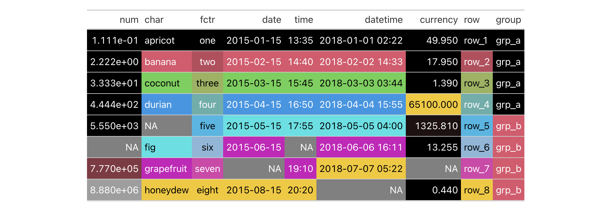
What's happened is that data_color() applies background colors to all cells
of every column with the default palette in R (accessed through palette()).
The default method for applying color is "auto", where numeric values will
use the "numeric" method and character or factor values will use the
"factor" method. The text color undergoes an automatic modification that
maximizes contrast (since autocolor_text is TRUE by default).
You can use any of the available method keywords and gt will only apply
color to the compatible values. Let's use the "numeric" method and supply
palette values of "red" and "green".
exibble |>
  gt() |>
  data_color(
    method = "numeric",
    palette = c("red", "green")
  )
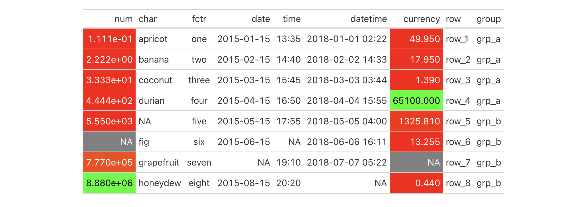
With those options in place we see that only the numeric columns num and
currency received color treatments. Moreover, the palette colors were
mapped to the lower and upper limits of the data in each column; interpolated
colors were used for the values in between the numeric limits of the two
columns.
We can constrain the cells to which coloring will be applied with the
columns and rows arguments. Further to this, we can manually set the
limits of the data with the domain argument (which is preferable in most
cases). Here, the domain will be set as domain = c(0, 50).
exibble |>
  gt() |>
  data_color(
    columns = currency,
    rows = currency < 50,
    method = "numeric",
    palette = c("red", "green"),
    domain = c(0, 50)
  )

We can use any of the palettes available in the RColorBrewer and
viridis packages. Let's make a new gt table from a subset of the
countrypops dataset. Then, through data_color(), we'll apply coloring
to the population column with the "numeric" method, use a domain between
2.5 and 3.4 million, and specify palette = "viridis".
countrypops |>
  dplyr::select(-contains("code")) |>
  dplyr::filter(
    country_name == "Bangladesh",
    year %in% 2012:2021
  ) |>
  gt() |>
  data_color(
    columns = population,
    method = "numeric",
    palette = "viridis",
    domain = c(150E6, 170E6),
    reverse = TRUE
  )

We can alternatively use the fn argument for supplying the scales-based
function scales::col_numeric(). That function call will itself return a
function (which is what the fn argument actually requires) that takes a
vector of numeric values and returns color values. Here is an alternate
version of the code that returns the same table as in the previous example.
countrypops |>
  dplyr::select(-contains("code")) |>
  dplyr::filter(
    country_name == "Bangladesh",
    year %in% 2012:2021
  ) |>
  gt() |>
  data_color(
    columns = population,
    fn = scales::col_numeric(
      palette = "viridis",
      domain = c(150E6, 170E6),
      reverse = TRUE
    )
  )
Using your own function in fn can be very useful if you want to make use of
specialized arguments in the scales::col_*() functions. You could even
supply your own specialized function for performing complex colorizing
treatments!
data_color() has a way to apply colorization indirectly to
other columns. That is, you can apply colors to a column different from the
one used to generate those specific colors. The trick is to use the
target_columns argument. Let's do this with a more complete
countrypops-based table example.
countrypops |>
  dplyr::filter(country_code_3 %in% c("FRA", "GBR")) |>
  dplyr::filter(year %% 10 == 0) |>
  dplyr::select(-contains("code")) |>
  dplyr::mutate(color = "") |>
  gt(groupname_col = "country_name") |>
  fmt_integer(columns = population) |>
  data_color(
    columns = population,
    target_columns = color,
    method = "numeric",
    palette = "viridis",
    domain = c(4E7, 7E7)
  ) |>
  cols_label(
    year = "",
    population = "Population",
    color = ""
  ) |>
  opt_vertical_padding(scale = 0.65)

When specifying a single column in columns we can use as many
target_columns values as we want. Let's make another countrypops-based
table where we map the generated colors from the year column to all columns
in the table. This time, the palette used is "inferno" (also from the
viridis package).
countrypops |>
  dplyr::filter(country_code_3 %in% c("FRA", "GBR", "ITA")) |>
  dplyr::select(-contains("code")) |>
  dplyr::filter(year %% 5 == 0) |>
  tidyr::pivot_wider(
    names_from = "country_name",
    values_from = "population"
  ) |>
  gt() |>
  fmt_integer(columns = c(everything(), -year)) |>
  cols_width(
    year ~ px(80),
    everything() ~ px(160)
  ) |>
  opt_all_caps() |>
  opt_vertical_padding(scale = 0.75) |>
  opt_horizontal_padding(scale = 3) |>
  data_color(
    columns = year,
    target_columns = everything(),
    palette = "inferno"
  ) |>
  tab_options(
    table_body.hlines.style = "none",
    column_labels.border.top.color = "black",
    column_labels.border.bottom.color = "black",
    table_body.border.bottom.color = "black"
  )

Now, it's time to use pizzaplace to create a gt table. The color
palette to be used is the "ggsci::red_material" one (it's in the ggsci
R package but also obtainable from the paletteer package).
Colorization will be applied to the to the sold and income columns. We
don't have to specify those in columns because those are the only columns
in the table. Also, the domain is not set here. We'll use the bounds of the
available data in each column.
pizzaplace |>
  dplyr::group_by(type, size) |>
  dplyr::summarize(
    sold = dplyr::n(),
    income = sum(price),
    .groups = "drop_last"
  ) |>
  dplyr::group_by(type) |>
  dplyr::mutate(f_sold = sold / sum(sold)) |>
  dplyr::mutate(size = factor(
    size, levels = c("S", "M", "L", "XL", "XXL"))
  ) |>
  dplyr::arrange(type, size) |>
  gt(
    rowname_col = "size",
    groupname_col = "type"
  ) |>
  fmt_percent(
    columns = f_sold,
    decimals = 1
  ) |>
  cols_merge(
    columns = c(size, f_sold),
    pattern = "{1} ({2})"
  ) |>
  cols_align(align = "left", columns = stub()) |>
  data_color(
    method = "numeric",
    palette = "ggsci::red_material"
  )

Colorization can occur in a row-wise manner. The key to making that happen is
by using direction = "row". Let's use the sza dataset to make a gt
table. Then, color will be applied to values across each 'month' of data in
that table. This is useful when not setting a domain as the bounds of each
row will be captured, coloring each cell with values relative to the range.
The palette is "PuOr" from the RColorBrewer package (only the name
here is required).
sza |>
  dplyr::filter(latitude == 20 & tst <= "1200") |>
  dplyr::select(-latitude) |>
  dplyr::filter(!is.na(sza)) |>
  tidyr::pivot_wider(
    names_from = tst,
    values_from = sza,
    names_sort = TRUE
  ) |>
  gt(rowname_col = "month") |>
  sub_missing(missing_text = "") |>
  data_color(
    direction = "row",
    palette = "PuOr",
    na_color = "white"
  )

Notice that na_color = "white" was used, and this avoids the appearance of
gray cells for the missing values (we also removed the "NA" text with
sub_missing(), opting for empty strings).
Function ID
3-37
Function Introduced
v0.2.0.5 (March 31, 2020)
See Also
Other data formatting functions:
fmt(),
fmt_auto(),
fmt_bins(),
fmt_bytes(),
fmt_chem(),
fmt_country(),
fmt_currency(),
fmt_date(),
fmt_datetime(),
fmt_duration(),
fmt_email(),
fmt_engineering(),
fmt_flag(),
fmt_fraction(),
fmt_icon(),
fmt_image(),
fmt_index(),
fmt_integer(),
fmt_markdown(),
fmt_number(),
fmt_number_si(),
fmt_partsper(),
fmt_passthrough(),
fmt_percent(),
fmt_roman(),
fmt_scientific(),
fmt_spelled_num(),
fmt_tf(),
fmt_time(),
fmt_units(),
fmt_url(),
sub_large_vals(),
sub_missing(),
sub_small_vals(),
sub_values(),
sub_zero()
Provide a vector of sensible system fonts for use with gt tables
Description
The vector of fonts given by default_fonts() can be safely used with a
gt table rendered as HTML since the font stack is expected to be
available across a wide set of systems. We can always specify additional
fonts to use and place them higher in precedence order, done through
prepending to this vector (i.e., this font stack should be placed after that
to act as a set of fallbacks).
This vector of fonts is useful when specifying font values inside
cell_text() (itself usable in tab_style() or tab_style_body()). If
using opt_table_font() (which also has a font argument), we probably
don't need to specify this vector of fonts since that function prepends font
names (this is handled by its add option, which is TRUE by default).
Usage
default_fonts()default_fonts()
Value
A character vector of font names.
Examples
Let's use the exibble dataset to create a simple, two-column gt table
(keeping only the char and time columns). Attempting to modify the fonts
used for the time column is much safer if default_fonts() is appended to
the end of the font listing inside cell_text(). What will happen, since
the "Comic Sansa" and "Menloa" fonts shouldn't exist, is that we'll get
exibble |>
  dplyr::select(char, time) |>
  gt() |>
  tab_style(
    style = cell_text(
      font = c("Comic Sansa", "Menloa", default_fonts())
    ),
    locations = cells_body(columns = time)
  )

Function ID
8-32
Function Introduced
v0.2.2 (August 5, 2020)
See Also
Other helper functions:
adjust_luminance(),
cell_borders(),
cell_fill(),
cell_text(),
currency(),
escape_latex(),
from_column(),
google_font(),
gt_latex_dependencies(),
html(),
latex(),
md(),
nanoplot_options(),
pct(),
px(),
random_id(),
row_group(),
stub(),
system_fonts(),
unit_conversion()
Perform LaTeX escaping
Description
Text may contain several characters with special meanings in LaTeX.
escape_latex() will transform a character vector so that it is safe to use
within LaTeX tables.
Usage
escape_latex( text, unicode_conversion = getOption("gt.latex.unicode_convert", default = FALSE) )escape_latex( text, unicode_conversion = getOption("gt.latex.unicode_convert", default = FALSE) )
Arguments
text |
LaTeX text
A character vector containing the text that is to be LaTeX-escaped. |
unicode_conversion |
Boolean
A boolean value indicating whether unicode in text should be turned into LaTeX. |
Value
A character vector.
Function ID
8-29
Function Introduced
v0.2.0.5 (March 31, 2020)
See Also
Other helper functions:
adjust_luminance(),
cell_borders(),
cell_fill(),
cell_text(),
currency(),
default_fonts(),
from_column(),
google_font(),
gt_latex_dependencies(),
html(),
latex(),
md(),
nanoplot_options(),
pct(),
px(),
random_id(),
row_group(),
stub(),
system_fonts(),
unit_conversion()
A toy example tibble for testing with gt: exibble
Description
This tibble contains data of a few different classes, which makes it
well-suited for quick experimentation with the functions in this package. It
contains only eight rows with numeric, character, and factor columns. The
last 4 rows contain NA values in the majority of this tibble's columns (1
missing value per column). The date, time, and datetime columns are
character-based dates/times in the familiar ISO 8601 format. The row and
group columns provide for unique rownames and two groups (grp_a and
grp_b) for experimenting with the gt() function's rowname_col and
groupname_col arguments.
Usage
exibbleexibble
Format
A tibble with 8 rows and 9 variables:
- num
-
A numeric column ordered with increasingly larger values.
- char
-
A character column composed of names of fruits from
atoh. - fctr
-
A factor column with numbers from
1to8, written out. - date, time, datetime
-
Character columns with dates, times, and datetimes.
- currency
-
A numeric column that is useful for testing currency-based formatting.
- row
-
A character column in the format
row_Xwhich can be useful for testing with row labels in a table stub. - group
-
A character column with four
grp_avalues and fourgrp_bvalues which can be useful for testing tables that contain row groups.
Dataset ID and Badge
DATA-6

Dataset Introduced
v0.2.0.5 (March 31, 2020)
See Also
Other datasets:
constants,
countrypops,
films,
gibraltar,
gtcars,
illness,
metro,
nuclides,
peeps,
photolysis,
pizzaplace,
reactions,
rx_addv,
rx_adsl,
sp500,
sza,
towny
Examples
exibbleexibble
Extract the table body from a gt object
Description
We can extract the body of a gt table, even at various stages of its
rendering, from a gt_tbl object using extract_body(). By default, the
data frame returned will have gone through all of the build stages but we
can intercept the table body after a certain build stage. Here are the eight
different build stages and some notes about each:
-
"init": the body table is initialized here, entirely withNAvalues. It's important to note that all columns of the are of thecharactertype in this first stage. And all columns remain in the same order as the input data table. -
"fmt_applied": Any cell values that have had formatting applied to them are migrated to the body table. All other cells remain asNAvalues. Depending on theoutputtype, the formatting may also be different. -
"sub_applied": Any cell values that have had substitution functions applied to them (whether or not they were previously formatted) are migrated to the body table or modified in place (if formatted). All cells that had neither been formatted nor undergone substitution remain asNAvalues. -
"unfmt_included": All cells that either didn't have any formatting or any substitution operations applied are migrated to the body table.NAvalues now become the string"NA", so, there aren't any true missing values in this body table. -
"cols_merged": The result of column-merging operations (throughcols_merge()and related functions) is materialized here. Columns that were asked to be hidden will be present here (i.e., hiding columns doesn't remove them from the body table). -
"body_reassembled": Though columns do not move positions rows can move to different positions, and this is usually due to migration to different row groups. At this stage, rows will be in the finalized order that is seen in the associated display table. -
"text_transformed": Varioustext_*()functions in gt can operate on body cells (now fully formatted at this stage) and return transformed character values. After this stage, the effects of those functions are apparent. -
"footnotes_attached": Footnote marks are attached to body cell values (either on the left or right of the content). This stage performs said attachment.
Usage
extract_body( data, build_stage = NULL, incl_hidden_cols = FALSE, incl_stub_cols = TRUE, ..., output = c("html", "latex", "rtf", "word", "grid") )extract_body( data, build_stage = NULL, incl_hidden_cols = FALSE, incl_stub_cols = TRUE, ..., output = c("html", "latex", "rtf", "word", "grid") )
Arguments
data |
The gt table data object
This is the gt table object that is commonly created through use of the
|
build_stage |
The build stage of the formatted R data frame
When a gt undergoes rendering, the body of the table proceeds through
several build stages. Providing a single stage name will yield a data frame
that has been extracted after completed that stage. Here are the build
stages in order: (1) |
|
Should hidden columns be included?
Certain columns may be hidden from final display via |
|
incl_stub_cols |
Should stub columns be included?
Any stub columns in the gt object (which may consist of a grouping
column and a column for row labels) are included in the extracted data for
clarity but clearly marked with the names |
... |
These dots are for future extensions and must be empty. |
output |
Output format
The output format of the resulting data frame. This can either be
|
Value
A data frame or tibble object containing the table body.
Examples
Use a modified version of sp500 the dataset to create a gt table with
row groups and row labels. Formatting will be applied to the date- and
currency-based columns.
gt_tbl <-
  sp500 |>
  dplyr::filter(date >= "2015-01-05" & date <= "2015-01-16") |>
  dplyr::arrange(date) |>
  dplyr::mutate(week = paste0("W", strftime(date, format = "%V"))) |>
  dplyr::select(-adj_close, -volume) |>
  gt(
    rowname_col = "date",
    groupname_col = "week"
  ) |>
  fmt_date(columns = date, date_style = "day_month_year") |>
  fmt_currency(columns = c(open, high, low, close)) |>
  cols_hide(columns = c(high, low))
gt_tbl

Using extract_body() on the gt object (gt_tbl) will provide us with
a tibble that contains the fully built data cells for the output context
(in this case, "html").
extract_body(gt_tbl)
#> # A tibble: 10 x 4
#>    `::group_id::` `::rowname::`   open      close
#>    <chr>          <chr>           <chr>     <chr>
#>  1 W02            5 January 2015  $2,054.44 $2,020.58
#>  2 W02            6 January 2015  $2,022.15 $2,002.61
#>  3 W02            7 January 2015  $2,005.55 $2,025.90
#>  4 W02            8 January 2015  $2,030.61 $2,062.14
#>  5 W02            9 January 2015  $2,063.45 $2,044.81
#>  6 W03            12 January 2015 $2,046.13 $2,028.26
#>  7 W03            13 January 2015 $2,031.58 $2,023.03
#>  8 W03            14 January 2015 $2,018.40 $2,011.27
#>  9 W03            15 January 2015 $2,013.75 $1,992.67
#> 10 W03            16 January 2015 $1,992.25 $2,019.42
To provide us with a better frame of reference, the grouping and row label
values are provided as the first columns in the returned output. We could
suppress those in the output by setting incl_stub_cols = FALSE.
extract_body(gt_tbl, incl_stub_cols = FALSE)
#> # A tibble: 10 x 2
#>    open      close
#>    <chr>     <chr>
#>  1 $2,054.44 $2,020.58
#>  2 $2,022.15 $2,002.61
#>  3 $2,005.55 $2,025.90
#>  4 $2,030.61 $2,062.14
#>  5 $2,063.45 $2,044.81
#>  6 $2,046.13 $2,028.26
#>  7 $2,031.58 $2,023.03
#>  8 $2,018.40 $2,011.27
#>  9 $2,013.75 $1,992.67
#> 10 $1,992.25 $2,019.42
The high and low columns were hidden via cols_hide() and so they
won't be shown in the returned data unless we use incl_hidden_cols = TRUE.
extract_body(
  gt_tbl,
  incl_stub_cols = FALSE,
  incl_hidden_cols = TRUE
)
#> # A tibble: 10 x 4
#>    open      high      low       close
#>    <chr>     <chr>     <chr>     <chr>
#>  1 $2,054.44 $2,054.44 $2,017.34 $2,020.58
#>  2 $2,022.15 $2,030.25 $1,992.44 $2,002.61
#>  3 $2,005.55 $2,029.61 $2,005.55 $2,025.90
#>  4 $2,030.61 $2,064.08 $2,030.61 $2,062.14
#>  5 $2,063.45 $2,064.43 $2,038.33 $2,044.81
#>  6 $2,046.13 $2,049.30 $2,022.58 $2,028.26
#>  7 $2,031.58 $2,056.93 $2,008.25 $2,023.03
#>  8 $2,018.40 $2,018.40 $1,988.44 $2,011.27
#>  9 $2,013.75 $2,021.35 $1,991.47 $1,992.67
#> 10 $1,992.25 $2,020.46 $1,988.12 $2,019.42
Function ID
13-7
Function Introduced
v0.10.0 (October 7, 2023)
See Also
Other table export functions:
as_gtable(),
as_latex(),
as_raw_html(),
as_rtf(),
as_word(),
extract_cells(),
extract_summary(),
gtsave()
Extract a vector of formatted cells from a gt object
Description
Get a vector of cell data from a gt_tbl object. The output vector will have
cell data formatted in the same way as the table.
Usage
extract_cells( data, columns, rows = everything(), output = c("auto", "plain", "html", "latex", "rtf", "word", "grid") )extract_cells( data, columns, rows = everything(), output = c("auto", "plain", "html", "latex", "rtf", "word", "grid") )
Arguments
data |
The gt table data object
This is the gt table object that is commonly created through use of the
|
columns |
Columns to target
Can either be a series of column names provided in |
rows |
Rows to target
In conjunction with |
output |
Output format
The output style of the resulting character vector. This can either be
|
Value
A vector of cell data extracted from a gt table.
Examples
Let's create a gt table with the exibble dataset to use in the next
few examples:
gt_tbl <- gt(exibble, rowname_col = "row", groupname_col = "group")
We can extract a cell from the table with the extract_cells() function.
This is done by providing a column and a row intersection:
extract_cells(gt_tbl, columns = num, row = 1)
#> [1] "1.111e-01"
Multiple cells can be extracted. Let's get the first four cells from the
char column.
extract_cells(gt_tbl, columns = char, rows = 1:4)
#> [1] "apricot" "banana" "coconut" "durian"
We can format cells and expect that the formatting is fully retained after extraction.
gt_tbl |>
  fmt_number(columns = num, decimals = 2) |>
  extract_cells(columns = num, rows = 1)
#> [1] "0.11"
Function ID
13-9
Function Introduced
v0.8.0 (November 16, 2022)
See Also
Other table export functions:
as_gtable(),
as_latex(),
as_raw_html(),
as_rtf(),
as_word(),
extract_body(),
extract_summary(),
gtsave()
Extract a summary list from a gt object
Description
Get a list of summary row data frames from a gt_tbl object where summary
rows were added via summary_rows(). The output data frames contain the
group_id and rowname columns, whereby rowname contains descriptive stub
labels for the summary rows.
Usage
extract_summary(data)extract_summary(data)
Arguments
data |
The gt table data object
This is the gt table object that is commonly created through use of the
|
Value
A list of data frames containing summary data.
Examples
Use a modified version of sp500 the dataset to create a gt table with
row groups and row labels. Create summary rows labeled as min, max, and
avg for every row group with summary_rows(). Then, extract the summary
rows as a list object.
summary_extracted <-
  sp500 |>
  dplyr::filter(date >= "2015-01-05" & date <="2015-01-30") |>
  dplyr::arrange(date) |>
  dplyr::mutate(week = paste0("W", strftime(date, format = "%V"))) |>
  dplyr::select(-adj_close, -volume) |>
  gt(
    rowname_col = "date",
    groupname_col = "week"
  ) |>
  summary_rows(
    groups = everything(),
    columns = c(open, high, low, close),
    fns = list(
      min = ~min(.),
      max = ~max(.),
      avg = ~mean(.)
    ),
  ) |>
  extract_summary()

summary_extracted
#> $summary_df_data_list
#> $summary_df_data_list$W02
#> # A tibble: 3 x 9
#>   group_id row_id rowname  date  open  high   low close  week
#>   <chr>    <chr>  <chr>   <dbl> <dbl> <dbl> <dbl> <dbl> <dbl>
#> 1 W02      min    min        NA 2006. 2030. 1992. 2003.    NA
#> 2 W02      max    max        NA 2063. 2064. 2038. 2062.    NA
#> 3 W02      avg    avg        NA 2035. 2049. 2017. 2031.    NA
#>
#> $summary_df_data_list$W03
#> # A tibble: 3 x 9
#>   group_id row_id rowname  date  open  high   low close  week
#>   <chr>    <chr>  <chr>   <dbl> <dbl> <dbl> <dbl> <dbl> <dbl>
#> 1 W03      min    min        NA 1992. 2018. 1988. 1993.    NA
#> 2 W03      max    max        NA 2046. 2057. 2023. 2028.    NA
#> 3 W03      avg    avg        NA 2020. 2033. 2000. 2015.    NA
#>
#> $summary_df_data_list$W04
#> # A tibble: 3 x 9
#>   group_id row_id rowname  date  open  high   low close  week
#>   <chr>    <chr>  <chr>   <dbl> <dbl> <dbl> <dbl> <dbl> <dbl>
#> 1 W04      min    min        NA 2020. 2029. 2004. 2023.    NA
#> 2 W04      max    max        NA 2063. 2065. 2051. 2063.    NA
#> 3 W04      avg    avg        NA 2035. 2049. 2023. 2042.    NA
#>
#> $summary_df_data_list$W05
#> # A tibble: 3 x 9
#>   group_id row_id rowname  date  open  high   low close  week
#>   <chr>    <chr>  <chr>   <dbl> <dbl> <dbl> <dbl> <dbl> <dbl>
#> 1 W05      min    min        NA 2002. 2023. 1989. 1995.    NA
#> 2 W05      max    max        NA 2050. 2058. 2041. 2057.    NA
#> 3 W05      avg    avg        NA 2030. 2039. 2009. 2021.    NA
Use the summary list to make a new gt table. The key thing is to use
dplyr::bind_rows() and then pass the tibble to gt().
summary_extracted |>
  unlist(recursive = FALSE) |>
  dplyr::bind_rows() |>
  gt(groupname_col = "group_id") |>
  cols_hide(columns = row_id)
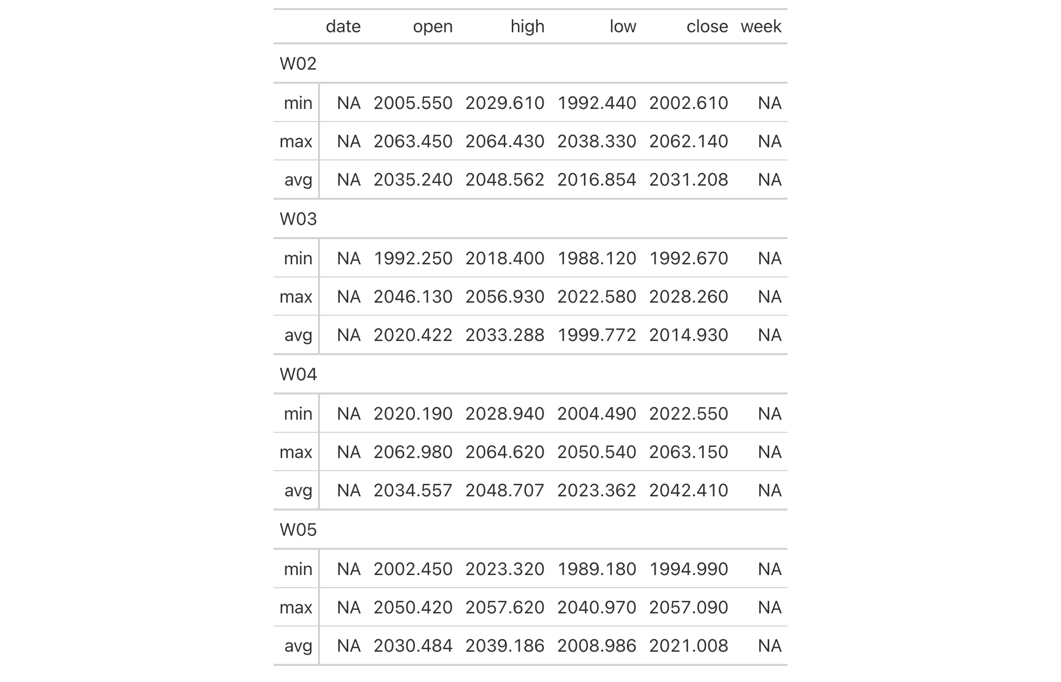
Function ID
13-8
Function Introduced
v0.2.0.5 (March 31, 2020)
See Also
Other table export functions:
as_gtable(),
as_latex(),
as_raw_html(),
as_rtf(),
as_word(),
extract_body(),
extract_cells(),
gtsave()
Feature films in competition at the Cannes Film Festival
Description
Each entry in the films is a feature film that appeared in the official
selection during a festival year (starting in 1946 and active to the present
day). The year column refers to the year of the festival and this figure
doesn't always coincide with the release year of the film. The film's title
reflects the most common title of the film in English, where the
original_title column provides the title of the film in its spoken language
(transliterated to Roman script where necessary).
Usage
filmsfilms
Format
A tibble with 1,873 rows and 8 variables:
- year
-
The year of the festival in which the film was in competition.
- title,original_title
-
The
titlefield provides the film title used for English-speaking audiences. Theoriginal_titlefield is populated whentitlediffers greatly from the non-English original. - director
-
The director or set of co-directors for the film. Multiple directors are separated by a comma.
- languages
-
The languages spoken in the film in the order of appearance. This consists of ISO 639 language codes (primarily as two-letter codes, but using three-letter codes where necessary).
- countries_of_origin
-
The country or countries of origin for the production. Here, 2-letter ISO 3166-1 country codes (set in uppercase) are used.
- run_time
-
The run time of the film in hours and minutes. This is given as a string in the format
[x]h [y]m. - imdb_url
-
The URL of the film's information page in the Internet Movie Database (IMDB).
Dataset ID and Badge
DATA-9

Dataset Introduced
v0.11.0 (July 9, 2024)
See Also
Other datasets:
constants,
countrypops,
exibble,
gibraltar,
gtcars,
illness,
metro,
nuclides,
peeps,
photolysis,
pizzaplace,
reactions,
rx_addv,
rx_adsl,
sp500,
sza,
towny
Examples
dplyr::glimpse(films)dplyr::glimpse(films)
Set a column format with a formatter function
Description
fmt() provides a way to execute custom formatting functionality with raw
data values in a way that can consider all output contexts.
Along with the columns and rows arguments that provide some precision in
targeting data cells, the fns argument allows you to define one or more
functions for manipulating the raw data.
If providing a single function to fns, the recommended format is in the
form: fns = function(x) .... This single function will format the targeted
data cells the same way regardless of the output format (e.g., HTML, LaTeX,
RTF).
If you require formatting of x that depends on the output format, a list of
functions can be provided for the html, latex, rtf, and default
contexts. This can be in the form of fns = list(html = function(x) ..., latex = function(x) ..., default = function(x) ...). In this
multiple-function case, we recommended including the default function as a
fallback if all contexts aren't provided.
Usage
fmt(data, columns = everything(), rows = everything(), compat = NULL, fns)fmt(data, columns = everything(), rows = everything(), compat = NULL, fns)
Arguments
data |
The gt table data object
This is the gt table object that is commonly created through use of the
|
columns |
Columns to target
Can either be a series of column names provided in |
rows |
Rows to target
In conjunction with |
compat |
Formatting compatibility
An optional vector that provides the compatible classes for the formatting.
By default this is |
fns |
Formatting functions
Either a single formatting function or a named list of functions. Can also
be anonymous functions, in both base R ( |
Value
An object of class gt_tbl.
Examples
Use the exibble dataset to create a gt table. We'll format the
numeric values in the num column with fmt(). We supply a functions to
the fns argument. This supplied function will take values in the
column (x), multiply them by 1000, and exclose them in single quotes.
exibble |>
  dplyr::select(-row, -group) |>
  gt() |>
  fmt(
    columns = num,
    fns = function(x) {
      paste0("'", x * 1000, "'")
    }
  )
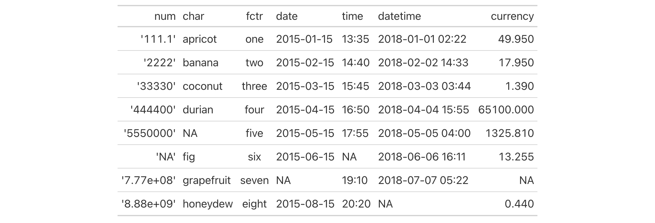
Function ID
3-31
Function Introduced
v0.2.0.5 (March 31, 2020)
See Also
Other data formatting functions:
data_color(),
fmt_auto(),
fmt_bins(),
fmt_bytes(),
fmt_chem(),
fmt_country(),
fmt_currency(),
fmt_date(),
fmt_datetime(),
fmt_duration(),
fmt_email(),
fmt_engineering(),
fmt_flag(),
fmt_fraction(),
fmt_icon(),
fmt_image(),
fmt_index(),
fmt_integer(),
fmt_markdown(),
fmt_number(),
fmt_number_si(),
fmt_partsper(),
fmt_passthrough(),
fmt_percent(),
fmt_roman(),
fmt_scientific(),
fmt_spelled_num(),
fmt_tf(),
fmt_time(),
fmt_units(),
fmt_url(),
sub_large_vals(),
sub_missing(),
sub_small_vals(),
sub_values(),
sub_zero()
Automatically format column data according to their values
Description
fmt_auto() will automatically apply formatting of various types in a way
that best suits the data table provided. The function will attempt to format
numbers such that they are condensed to an optimal width, either with
scientific notation or large-number suffixing. Currency values are detected
by currency codes embedded in the column name and formatted in the correct
way. Although the functionality here is comprehensive it's still possible to
reduce the scope of automatic formatting with the scope argument and also
by choosing a subset of columns and rows to which the formatting will be applied.
Usage
fmt_auto( data, columns = everything(), rows = everything(), scope = c("numbers", "currency"), lg_num_pref = c("sci", "suf"), locale = NULL )fmt_auto( data, columns = everything(), rows = everything(), scope = c("numbers", "currency"), lg_num_pref = c("sci", "suf"), locale = NULL )
Arguments
data |
The gt table data object
This is the gt table object that is commonly created through use of the
|
columns |
Columns to target
Can either be a series of column names provided in |
rows |
Rows to target
In conjunction with |
scope |
Scope of automatic formatting
By default, the function will format both |
lg_num_pref |
Large-number preference
When large numbers are present, there can be a fixed preference toward how
they are formatted. Choices are scientific notation for very small and very
large values ( |
locale |
Locale identifier
An optional locale identifier that can be used for formatting values
according to the locale's rules. Examples include |
Value
An object of class gt_tbl.
Examples
Use the exibble dataset to create a gt table. Format all of the
columns automatically with the fmt_auto() function.
exibble |>
  gt() |>
  fmt_auto()
Let's now use the countrypops dataset to create another gt table.
We'll again use fmt_auto() to automatically format all columns but this
time the choice will be made to opt for large-number suffixing instead of
scientific notation. This is done by using the lg_num_pref = "suf" option.
countrypops |>
  dplyr::select(country_code_3, year, population) |>
  dplyr::filter(country_code_3 %in% c("CHN", "IND", "USA", "PAK", "IDN")) |>
  dplyr::filter(year > 1975 & year %% 5 == 0) |>
  tidyr::pivot_wider(names_from = year, values_from = population) |>
  dplyr::arrange(desc(`2020`)) |>
  gt(rowname_col = "country_code_3") |>
  fmt_auto(lg_num_pref = "suf")

Function ID
3-30
Function Introduced
v0.9.0 (Mar 31, 2023)
See Also
Other data formatting functions:
data_color(),
fmt(),
fmt_bins(),
fmt_bytes(),
fmt_chem(),
fmt_country(),
fmt_currency(),
fmt_date(),
fmt_datetime(),
fmt_duration(),
fmt_email(),
fmt_engineering(),
fmt_flag(),
fmt_fraction(),
fmt_icon(),
fmt_image(),
fmt_index(),
fmt_integer(),
fmt_markdown(),
fmt_number(),
fmt_number_si(),
fmt_partsper(),
fmt_passthrough(),
fmt_percent(),
fmt_roman(),
fmt_scientific(),
fmt_spelled_num(),
fmt_tf(),
fmt_time(),
fmt_units(),
fmt_url(),
sub_large_vals(),
sub_missing(),
sub_small_vals(),
sub_values(),
sub_zero()
Format column data containing bin/interval information
Description
When using cut() (or other functions that use it in some way)
you get bins that can look like this: "(0,10]", "(10,15]", "(15,20]",
"(20,40]". This interval notation expresses the lower and upper limits of
each range. The square or round brackets define whether each of the endpoints
are included in the range ([/] for inclusion, (/) for exclusion).
Should bins of this sort be present in a table, the fmt_bins() function can
be used to format that syntax to a form that presents better in a display
table. It's possible to format the values of the intervals with the fmt
argument, and, the separator can be modified with the sep argument.
Usage
fmt_bins( data, columns = everything(), rows = everything(), sep = "--", fmt = NULL )fmt_bins( data, columns = everything(), rows = everything(), sep = "--", fmt = NULL )
Arguments
data |
The gt table data object
This is the gt table object that is commonly created through use of the
|
columns |
Columns to target
Can either be a series of column names provided in |
rows |
Rows to target
In conjunction with |
sep |
Separator between values
The separator text that indicates the values are ranged. The default value
of |
fmt |
Formatting expressions
An optional formatting expression in formula form. If used, the RHS of |
Value
An object of class gt_tbl.
Compatibility of formatting function with data values
fmt_bins() is compatible with body cells that are of the "character" or
"factor" types. Any other types of body cells are ignored during formatting.
This is to say that cells of incompatible data types may be targeted, but
there will be no attempt to format them.
Formatting expressions for fmt
We can supply a one-sided (RHS only) expression to fmt, and, several can be
provided in a list. The expression uses a formatting function (e.g.,
fmt_number(), fmt_currency(), etc.) and it must contain an initial .
that stands for the data object. If performing numeric formatting it might
look something like this:
fmt = ~ fmt_number(., decimals = 1, use_seps = FALSE)
Examples
Use the countrypops dataset to create a gt table. Before even getting
to the gt() call, we use cut() in conjunction with scales::breaks_log()
to create some highly customized bins. Consequently each country's population
in the 2021 year is assigned to a bin. These bins have a characteristic type
of formatting that can be used as input to fmt_bins(), and using that
formatting function allows us to customize the presentation of those ranges.
For instance, here we are formatting the left and right values of the ranges
with fmt_integer() (using formula syntax).
countrypops |>
  dplyr::filter(year == 2021) |>
  dplyr::select(country_code_2, population) |>
  dplyr::mutate(population_class = cut(
    population,
    breaks = scales::breaks_log(n = 20)(population)
    )
  ) |>
  dplyr::group_by(population_class) |>
  dplyr::summarize(
    count = dplyr::n(),
    countries = paste0(country_code_2, collapse = ",")
  ) |>
  dplyr::arrange(desc(population_class)) |>
  gt() |>
  fmt_flag(columns = countries) |>
  fmt_bins(
    columns = population_class,
    fmt = ~ fmt_integer(., suffixing = TRUE)
  ) |>
  cols_label(
    population_class = "Population Range",
    count = "",
    countries = "Countries"
  ) |>
  cols_width(
    population_class ~ px(150),
    count ~ px(50)
  ) |>
  tab_style(
    style = cell_text(style = "italic"),
    locations = cells_body(columns = count)
  )
Function ID
3-18
Function Introduced
v0.9.0 (Mar 31, 2023)
See Also
Other data formatting functions:
data_color(),
fmt(),
fmt_auto(),
fmt_bytes(),
fmt_chem(),
fmt_country(),
fmt_currency(),
fmt_date(),
fmt_datetime(),
fmt_duration(),
fmt_email(),
fmt_engineering(),
fmt_flag(),
fmt_fraction(),
fmt_icon(),
fmt_image(),
fmt_index(),
fmt_integer(),
fmt_markdown(),
fmt_number(),
fmt_number_si(),
fmt_partsper(),
fmt_passthrough(),
fmt_percent(),
fmt_roman(),
fmt_scientific(),
fmt_spelled_num(),
fmt_tf(),
fmt_time(),
fmt_units(),
fmt_url(),
sub_large_vals(),
sub_missing(),
sub_small_vals(),
sub_values(),
sub_zero()
Format values as bytes
Description
With numeric values in a gt table, we can transform those to values of
bytes with human readable units. fmt_bytes() allows for the
formatting of byte sizes to either of two common representations: (1) with
decimal units (powers of 1000, examples being "kB" and "MB"), and (2)
with binary units (powers of 1024, examples being "KiB" and "MiB").
It is assumed the input numeric values represent the number of bytes and automatic truncation of values will occur. The numeric values will be scaled to be in the range of 1 to <1000 and then decorated with the correct unit symbol according to the standard chosen. For more control over the formatting of byte sizes, we can use the following options:
-
decimals: choice of the number of decimal places, option to drop trailing zeros, and a choice of the decimal symbol
-
digit grouping separators: options to enable/disable digit separators and provide a choice of separator symbol
-
pattern: option to use a text pattern for decoration of the formatted values
-
locale-based formatting: providing a locale ID will result in number formatting specific to the chosen locale
Usage
fmt_bytes( data, columns = everything(), rows = everything(), standard = c("decimal", "binary"), decimals = 1, n_sigfig = NULL, drop_trailing_zeros = TRUE, drop_trailing_dec_mark = TRUE, use_seps = TRUE, min_sep_threshold = 1, pattern = "{x}", sep_mark = ",", dec_mark = ".", force_sign = FALSE, incl_space = TRUE, locale = NULL )fmt_bytes( data, columns = everything(), rows = everything(), standard = c("decimal", "binary"), decimals = 1, n_sigfig = NULL, drop_trailing_zeros = TRUE, drop_trailing_dec_mark = TRUE, use_seps = TRUE, min_sep_threshold = 1, pattern = "{x}", sep_mark = ",", dec_mark = ".", force_sign = FALSE, incl_space = TRUE, locale = NULL )
Arguments
data |
The gt table data object
This is the gt table object that is commonly created through use of the
|
columns |
Columns to target
Can either be a series of column names provided in |
rows |
Rows to target
In conjunction with |
standard |
Standard used to express byte sizes
The form of expressing large byte sizes is divided between: (1) decimal
units (powers of 1000; e.g., |
decimals |
Number of decimal places
This corresponds to the exact number of decimal places to use. A value
such as |
n_sigfig |
Number of significant figures
A option to format numbers to n significant figures. By default, this is
|
drop_trailing_zeros |
Drop any trailing zeros
A logical value that allows for removal of trailing zeros (those redundant zeros after the decimal mark). |
drop_trailing_dec_mark |
Drop the trailing decimal mark
A logical value that determines whether decimal marks should always appear
even if there are no decimal digits to display after formatting (e.g., |
use_seps |
Use digit group separators
An option to use digit group separators. The type of digit group separator
is set by |
min_sep_threshold |
Minimum digit threshold for grouping separators
The minimum number of digits required in the integer part of a number for
grouping separators to be applied. This parameter determines when digit
grouping begins based on the magnitude of values. The value |
pattern |
Specification of the formatting pattern
A formatting pattern that allows for decoration of the formatted value. The
formatted value is represented by the |
sep_mark |
Separator mark for digit grouping
The string to use as a separator between groups of digits. For example,
using |
dec_mark |
Decimal mark
The string to be used as the decimal mark. For example, using
|
force_sign |
Forcing the display of a positive sign
Should the positive sign be shown for positive numbers (effectively showing
a sign for all numbers except zero)? If so, use |
incl_space |
Include a space between the value and the units
An option for whether to include a space between the value and the units. The default is to use a space character for separation. |
locale |
Locale identifier
An optional locale identifier that can be used for formatting values
according to the locale's rules. Examples include |
Value
An object of class gt_tbl.
Compatibility of formatting function with data values
fmt_bytes() is compatible with body cells that are of the "numeric" or
"integer" types. Any other types of body cells are ignored during
formatting. This is to say that cells of incompatible data types may be
targeted, but there will be no attempt to format them.
Compatibility of arguments with the from_column() helper function
from_column() can be used with certain arguments of fmt_bytes() to obtain
varying parameter values from a specified column within the table. This means
that each row could be formatted a little bit differently. These arguments
provide support for from_column():
-
standard -
decimals -
n_sigfig -
drop_trailing_zeros -
drop_trailing_dec_mark -
use_seps -
pattern -
sep_mark -
dec_mark -
force_sign -
incl_space -
locale
Please note that for each of the aforementioned arguments, a from_column()
call needs to reference a column that has data of the correct type (this is
different for each argument). Additional columns for parameter values can be
generated with cols_add() (if not already present). Columns that contain
parameter data can also be hidden from final display with cols_hide().
Finally, there is no limitation to how many arguments the from_column()
helper is applied so long as the arguments belong to this closed set.
Adapting output to a specific locale
This formatting function can adapt outputs according to a provided locale
value. Examples include "en" for English (United States) and "fr" for
French (France). The use of a valid locale ID here means separator and
decimal marks will be correct for the given locale. Should any values be
provided in sep_mark or dec_mark, they will be overridden by the locale's
preferred values.
Note that a locale value provided here will override any global locale
setting performed in gt()'s own locale argument (it is settable there as
a value received by all other functions that have a locale argument). As a
useful reference on which locales are supported, we can call info_locales()
to view an info table.
Examples
Use a single column from the exibble dataset and create a simple gt
table. We'll use fmt_bytes() to format the num column to display as byte
sizes in the decimal standard.
exibble |>
  dplyr::select(num) |>
  gt() |>
  fmt_bytes()

Let's create an analogous table again by using fmt_bytes(),
this time showing byte sizes as binary values by using standard = "binary".
exibble |>
  dplyr::select(num) |>
  gt() |>
  fmt_bytes(standard = "binary")

Function ID
3-13
Function Introduced
v0.3.0 (May 12, 2021)
See Also
The vector-formatting version of this function: vec_fmt_bytes().
Other data formatting functions:
data_color(),
fmt(),
fmt_auto(),
fmt_bins(),
fmt_chem(),
fmt_country(),
fmt_currency(),
fmt_date(),
fmt_datetime(),
fmt_duration(),
fmt_email(),
fmt_engineering(),
fmt_flag(),
fmt_fraction(),
fmt_icon(),
fmt_image(),
fmt_index(),
fmt_integer(),
fmt_markdown(),
fmt_number(),
fmt_number_si(),
fmt_partsper(),
fmt_passthrough(),
fmt_percent(),
fmt_roman(),
fmt_scientific(),
fmt_spelled_num(),
fmt_tf(),
fmt_time(),
fmt_units(),
fmt_url(),
sub_large_vals(),
sub_missing(),
sub_small_vals(),
sub_values(),
sub_zero()
Format chemical formulas
Description
fmt_chem() lets you format chemical formulas or even chemical
reactions in the table body. Often the input text will be in a common form
representing single compounds (like "C2H4O", for acetaldehyde) but chemical
reactions can be used (e.g., 2CH3OH -> CH3OCH3 + H2O"). So long as the
text within the targeted cells conforms to gt's specialized chemistry
notation, the appropriate conversions will occur. Details pertaining to
chemistry notation can be found in the section entitled
How to use gt's chemistry notation.
Usage
fmt_chem(data, columns = everything(), rows = everything())fmt_chem(data, columns = everything(), rows = everything())
Arguments
data |
The gt table data object
This is the gt table object that is commonly created through use of the
|
columns |
Columns to target
Can either be a series of column names provided in |
rows |
Rows to target
In conjunction with |
Value
An object of class gt_tbl.
How to use gt's chemistry notation
The chemistry notation involves a shorthand of writing chemical formulas and chemical reactions, if needed. It should feel familiar in its basic usage and the more advanced typesetting tries to limit the amount of syntax needed. It's always best to show examples on usage:
-
"CH3O2"and"(NH4)2S"will render with subscripted numerals -
Charges can be expressed with terminating
"+"or"-", as in"H+"and"[AgCl2]-"; if any charges involve the use of a number, the following incantations could be used:"CrO4^2-","Fe^n+","Y^99+","Y^{99+}"(the final two forms produce equivalent output) -
Stoichiometric values can be included with whole values prepending formulas (e.g.,
"2H2O2") or by setting them off with a space, like this:"2 H2O2","0.5 H2O","1/2 H2O","(1/2) H2O" -
Certain standalone, lowercase letters or combinations thereof will be automatically stylized to fit conventions;
"NO_x"and"x Na(NH4)HPO4"will have italicized 'x' characters and you can always italicize letters by surrounding with"*"(as in"*n* H2O"or"*n*-C5H12") -
Chemical isotopes can be rendered using either of these two constructions preceding an element:
"^{227}_{90}Th"or"^227_90Th"; nuclides can be represented in a similar manner, here are two examples:"^{0}_{-1}n^{-}","^0_-1n-" -
Chemical reactions can use
"+"signs and a variety of reaction arrows: (1)"A -> B", (2)"A <- B", (3)"A <-> B", (4)"A <--> B", (5)"A <=> B", (6)"A <=>> B", or (7)"A <<=> B" -
Center dots (useful in addition compounds) can be added by using a single
"."or"*"character, surrounded by spaces; here are two equivalent examples"KCr(SO4)2 . 12 H2O"and"KCr(SO4)2 * 12 H2O" -
Single and double bonds can be shown by inserting a
"-"or"="between adjacent characters (i.e., these shouldn't be at the beginning or end of the markup); two examples:"C6H5-CHO","CH3CH=CH2" -
as with units notation, Greek letters can be inserted by surrounding the letter name with
":"; here's an example that describes the delta value of carbon-13:":delta: ^13C"
Examples
Let's use the reactions dataset and create a new gt table. The table
will be filtered down to only a few rows and columns. The column
cmpd_formula contains chemical formulas and the formatting of those will be
performed by fmt_chem(). Certain column labels with chemical names
(o3_k298 and no3_k298) can be handled within cols_label() by using
surrounding the text with "{{%"/"%}}".
reactions |>
  dplyr::filter(cmpd_type == "terminal monoalkene") |>
  dplyr::filter(grepl("^1-", cmpd_name)) |>
  dplyr::select(cmpd_name, cmpd_formula, ends_with("k298")) |>
  gt() |>
  tab_header(title = "Gas-phase reactions of selected terminal alkenes") |>
  tab_spanner(
    label = "Reaction Rate Constant at 298 K",
    columns = ends_with("k298")
  ) |>
  fmt_chem(columns = cmpd_formula) |>
  fmt_scientific() |>
  sub_missing() |>
  cols_label(
    cmpd_name = "Alkene",
    cmpd_formula = "Formula",
    OH_k298 = "OH",
    O3_k298 = "{{%O3%}}",
    NO3_k298 = "{{%NO3%}}",
    Cl_k298 = "Cl"
  ) |>
  opt_align_table_header(align = "left")

Taking just a few rows from the photolysis dataset, let's create a new
gt table. The cmpd_formula and products columns both contain text in
chemistry notation (the first has compounds, and the second column has the
products of photolysis reactions). These columns will be formatted by
fmt_chem(). The compound formulas will be merged with the compound
names with cols_merge().
photolysis |>
  dplyr::filter(cmpd_name %in% c(
    "hydrogen peroxide", "nitrous acid",
    "nitric acid", "acetaldehyde",
    "methyl peroxide", "methyl nitrate",
    "ethyl nitrate", "isopropyl nitrate"
  )) |>
  dplyr::select(-c(l, m, n, quantum_yield, type)) |>
  gt() |>
  tab_header(title = "Photolysis pathways of selected VOCs") |>
  fmt_chem(columns = c(cmpd_formula, products)) |>
  cols_nanoplot(
    columns = sigma_298_cm2,
    columns_x_vals = wavelength_nm,
    expand_x = c(200, 400),
    new_col_name = "cross_section",
    new_col_label = "Absorption Cross Section",
    options = nanoplot_options(
      show_data_points = FALSE,
      data_line_stroke_width = 4,
      data_line_stroke_color = "black",
      show_data_area = FALSE
    )
  ) |>
  cols_merge(
    columns = c(cmpd_name, cmpd_formula),
    pattern = "{1}, {2}"
  ) |>
  cols_label(
    cmpd_name = "Compound",
    products = "Products"
  ) |>
  opt_align_table_header(align = "left")

fmt_chem() can handle the typesetting of nuclide notation.
Let's take a subset of columns and rows from the nuclides dataset and
make a new gt table. The contents of the nuclide column contains
isotopes of hydrogen and carbon and this is placed in the table stub. Using
fmt_chem() makes it so that the subscripted and superscripted values are
properly formatted to the convention of formatting nuclides.
nuclides |>
  dplyr::filter(element %in% c("H", "C")) |>
  dplyr::mutate(nuclide = gsub("[0-9]+$", "", nuclide)) |>
  dplyr::select(nuclide, atomic_mass, half_life, decay_1, is_stable) |>
  gt(rowname_col = "nuclide") |>
  tab_header(title = "Isotopes of Hydrogen and Carbon") |>
  tab_stubhead(label = "Isotope") |>
  fmt_chem(columns = nuclide) |>
  fmt_scientific(columns = half_life) |>
  fmt_number(
    columns = atomic_mass,
    decimals = 4,
    scale_by = 1 / 1e6
  ) |>
  sub_missing(
    columns = half_life,
    rows = is_stable,
    missing_text = md("**STABLE**")
  ) |>
  sub_missing(columns = half_life, rows = !is_stable) |>
  sub_missing(columns = decay_1) |>
  data_color(
    columns = decay_1,
    target_columns = c(atomic_mass, half_life, decay_1),
    palette = "LaCroixColoR::PassionFruit",
    na_color = "white"
  ) |>
  cols_label_with(fn = function(x) tools::toTitleCase(gsub("_", " ", x))) |>
  cols_label(decay_1 = "Decay Mode") |>
  cols_width(
    stub() ~ px(70),
    c(atomic_mass, half_life, decay_1) ~ px(120)
  ) |>
  cols_hide(columns = c(is_stable)) |>
  cols_align(align = "center", columns = decay_1) |>
  opt_align_table_header(align = "left") |>
  opt_vertical_padding(scale = 0.5)

Function ID
3-21
Function Introduced
v0.11.0 (July 9, 2024)
See Also
Other data formatting functions:
data_color(),
fmt(),
fmt_auto(),
fmt_bins(),
fmt_bytes(),
fmt_country(),
fmt_currency(),
fmt_date(),
fmt_datetime(),
fmt_duration(),
fmt_email(),
fmt_engineering(),
fmt_flag(),
fmt_fraction(),
fmt_icon(),
fmt_image(),
fmt_index(),
fmt_integer(),
fmt_markdown(),
fmt_number(),
fmt_number_si(),
fmt_partsper(),
fmt_passthrough(),
fmt_percent(),
fmt_roman(),
fmt_scientific(),
fmt_spelled_num(),
fmt_tf(),
fmt_time(),
fmt_units(),
fmt_url(),
sub_large_vals(),
sub_missing(),
sub_small_vals(),
sub_values(),
sub_zero()
Generate country names from their corresponding country codes
Description
Tables that have comparable data between countries often need to have the
country name included. While this seems like a fairly simple task, being
consistent with country names is surprisingly difficult. The fmt_country()
function can help in this regard by supplying a country name based on a
2- or 3-letter ISO 3166-1 country code (e.g., Singapore has the "SG"
country code). The resulting country names have been obtained from the
Unicode CLDR (Common Locale Data Repository), which is a good source since
all country names are agreed upon by consensus. Furthermore, the country
names can be localized through the locale argument (either in this function
or through the initial gt() call).
Multiple country names can be included per cell by separating country codes
with commas (e.g., "RO,BM"). And it is okay if the codes are set in either
uppercase or lowercase letters. The sep argument allows for a common
separator to be applied between country names.
Usage
fmt_country( data, columns = everything(), rows = everything(), pattern = "{x}", sep = " ", locale = NULL )fmt_country( data, columns = everything(), rows = everything(), pattern = "{x}", sep = " ", locale = NULL )
Arguments
data |
The gt table data object
This is the gt table object that is commonly created through use of the
|
columns |
Columns to target
Can either be a series of column names provided in |
rows |
Rows to target
In conjunction with |
pattern |
Specification of the formatting pattern
A formatting pattern that allows for decoration of the formatted value. The
formatted value is represented by the |
sep |
Separator between country names
In the output of country names within a body cell, |
locale |
Locale identifier
An optional locale identifier that can be used for formatting values
according to the locale's rules. Examples include |
Value
An object of class gt_tbl.
Compatibility of formatting function with data values
fmt_country() function is compatible with body cells that are of the
"character" or "factor" types. Any other types of body cells are ignored
during formatting. This is to say that cells of incompatible data types may
be targeted, but there will be no attempt to format them.
Compatibility of arguments with the from_column() helper function
from_column() can be used with certain arguments of fmt_country() to
obtain varying parameter values from a specified column within the table.
This means that each row could be formatted a little bit differently. These
arguments provide support for from_column():
-
pattern -
sep -
locale
Please note that for each of the aforementioned arguments, a from_column()
call needs to reference a column that has data of the correct type (this is
different for each argument). Additional columns for parameter values can be
generated with cols_add() (if not already present). Columns that contain
parameter data can also be hidden from final display with cols_hide().
Finally, there is no limitation to how many arguments the from_column()
helper is applied so long as the arguments belong to this closed set.
Supported regions
The following 242 regions (most of which comprise countries) are supported
with names across 574 locales: "AD", "AE", "AF", "AG", "AI",
"AL", "AM", "AO", "AR", "AS", "AT", "AU", "AW", "AX",
"AZ", "BA", "BB", "BD", "BE", "BF", "BG", "BH", "BI",
"BJ", "BL", "BM", "BN", "BO", "BR", "BS", "BT", "BW",
"BY", "BZ", "CA", "CC", "CD", "CF", "CG", "CH", "CI",
"CK", "CL", "CM", "CN", "CO", "CR", "CU", "CV", "CW",
"CY", "CZ", "DE", "DJ", "DK", "DM", "DO", "DZ", "EC",
"EE", "EG", "EH", "ER", "ES", "ET", "EU", "FI", "FJ",
"FK", "FM", "FO", "FR", "GA", "GB", "GD", "GE", "GF",
"GG", "GH", "GI", "GL", "GM", "GN", "GP", "GQ", "GR",
"GS", "GT", "GU", "GW", "GY", "HK", "HN", "HR", "HT",
"HU", "ID", "IE", "IL", "IM", "IN", "IO", "IQ", "IR",
"IS", "IT", "JE", "JM", "JO", "JP", "KE", "KG", "KH",
"KI", "KM", "KN", "KP", "KR", "KW", "KY", "KZ", "LA",
"LB", "LC", "LI", "LK", "LR", "LS", "LT", "LU", "LV",
"LY", "MA", "MC", "MD", "ME", "MF", "MG", "MH", "MK",
"ML", "MM", "MN", "MO", "MP", "MQ", "MR", "MS", "MT",
"MU", "MV", "MW", "MX", "MY", "MZ", "NA", "NC", "NE",
"NF", "NG", "NI", "NL", "NO", "NP", "NR", "NU", "NZ",
"OM", "PA", "PE", "PF", "PG", "PH", "PK", "PL", "PM",
"PN", "PR", "PS", "PT", "PW", "PY", "QA", "RE", "RO",
"RS", "RU", "RW", "SA", "SB", "SC", "SD", "SE", "SG",
"SI", "SK", "SL", "SM", "SN", "SO", "SR", "SS", "ST",
"SV", "SX", "SY", "SZ", "TC", "TD", "TF", "TG", "TH",
"TJ", "TK", "TL", "TM", "TN", "TO", "TR", "TT", "TV",
"TW", "TZ", "UA", "UG", "US", "UY", "UZ", "VA", "VC",
"VE", "VG", "VI", "VN", "VU", "WF", "WS", "YE", "YT",
"ZA", "ZM", and "ZW".
Examples
The peeps dataset will be used to generate a small gt table
containing only the people born in the 1980s. The country column contains
3-letter country codes and those will be transformed to country names with
fmt_country().
peeps |>
  dplyr::filter(grepl("198", dob)) |>
  dplyr::select(name_given, name_family, country, dob) |>
  dplyr::arrange(country, name_family) |>
  gt() |>
  fmt_country(columns = country) |>
  cols_merge(columns = c(name_given, name_family)) |>
  opt_vertical_padding(scale = 0.5) |>
  tab_options(column_labels.hidden = TRUE)

Use the countrypops dataset to create a gt table. We will only
include a few columns and rows from that table. The country_code_3 column
has 3-letter country codes in the format required for fmt_country() and
using that function transforms the codes to country names.
countrypops |>
  dplyr::filter(year == 2021) |>
  dplyr::filter(grepl("^S", country_name)) |>
  dplyr::arrange(country_name) |>
  dplyr::select(-country_name, -year) |>
  dplyr::slice_head(n = 10) |>
  gt() |>
  fmt_integer() |>
  fmt_flag(columns = country_code_2) |>
  fmt_country(columns = country_code_3) |>
  cols_label(
    country_code_2 = "",
    country_code_3 = "Country",
    population = "Population (2021)"
  )

The country names derived from country codes can be localized. Let's
translate some of those country names into three different languages using
different locale values in separate calls of fmt_country().
countrypops |>
  dplyr::filter(year == 2021) |>
  dplyr::arrange(desc(population)) |>
  dplyr::filter(
    dplyr::row_number() > max(dplyr::row_number()) - 5 |
    dplyr::row_number() <= 5
  ) |>
  dplyr::select(
    country_code_fl = country_code_2,
    country_code_2a = country_code_2,
    country_code_2b = country_code_2,
    country_code_2c = country_code_2,
    population
  ) |>
  gt(rowname_col = "country_code_fl") |>
  fmt_integer() |>
  fmt_flag(columns = stub()) |>
  fmt_country(columns = ends_with("a")) |>
  fmt_country(columns = ends_with("b"), locale = "ja") |>
  fmt_country(columns = ends_with("c"), locale = "ar") |>
  cols_label(
    ends_with("a") ~ "`en`",
    ends_with("b") ~ "`ja`",
    ends_with("c") ~ "`ar`",
    population = "Population",
    .fn = md
  ) |>
  tab_spanner(
    label = "Country name in specified locale",
    columns = matches("2a|2b|2c")
  ) |>
  cols_align(align = "center", columns = matches("2a|2b|2c")) |>
  opt_horizontal_padding(scale = 2)

Let's make another gt table, this time using the films dataset. The
countries_of_origin column contains 2-letter country codes and some cells
contain multiple countries (separated by commas). We'll use fmt_country()
on that column and also specify that the rendered country names should be
separated by a comma and a space character. Also note that historical
country codes like "SU" ('USSR'), "CS" ('Czechoslovakia'), and "YU"
('Yugoslavia') are permitted as inputs for fmt_country().
films |>
  dplyr::filter(year == 1959) |>
  dplyr::select(
    contains("title"), run_time, director, countries_of_origin, imdb_url
  ) |>
  gt() |>
  tab_header(title = "Feature Films in Competition at the 1959 Festival") |>
  fmt_country(columns = countries_of_origin, sep = ", ") |>
  fmt_url(
    columns = imdb_url,
    label = fontawesome::fa("imdb", fill = "black")
  ) |>
  cols_merge(
    columns = c(title, original_title, imdb_url),
    pattern = "{1}<< ({2})>> {3}"
  ) |>
  cols_label(
    title = "Film",
    run_time = "Length",
    director = "Director",
    countries_of_origin = "Country"
  ) |>
  opt_vertical_padding(scale = 0.5) |>
  opt_table_font(stack = "classical-humanist", weight = "bold") |>
  opt_stylize(style = 1, color = "gray") |>
  tab_options(heading.title.font.size = px(26))

Country names can sometimes pair nicely with flag-based graphics. In this
example (using a different portion of the films dataset) we use
fmt_country() along with fmt_flag(). The formatted country names are then
merged into the same cells as the icons via cols_merge().
films |>
  dplyr::filter(director == "Jean-Pierre Dardenne, Luc Dardenne") |>
  dplyr::select(title, year, run_time, countries_of_origin) |>
  gt() |>
  tab_header(title = "In Competition Films by the Dardenne Bros.") |>
  cols_add(country_flag = countries_of_origin) |>
  fmt_flag(columns = country_flag) |>
  fmt_country(columns = countries_of_origin, sep = ", ") |>
  cols_merge(
    columns = c(countries_of_origin, country_flag),
    pattern = "{2}<br>{1}"
  ) |>
  tab_style(
    style = cell_text(size = px(9)),
    locations = cells_body(columns = countries_of_origin)
  ) |>
  cols_merge(columns = c(title, year), pattern = "{1} ({2})") |>
  opt_vertical_padding(scale = 0.5) |>
  opt_horizontal_padding(scale = 3) |>
  opt_table_font(font = google_font("PT Sans")) |>
  opt_stylize(style = 1, color = "blue") |>
  tab_options(
    heading.title.font.size = px(26),
    column_labels.hidden = TRUE
  )

Function ID
3-26
Function Introduced
v0.11.0 (July 9, 2024)
See Also
Other data formatting functions:
data_color(),
fmt(),
fmt_auto(),
fmt_bins(),
fmt_bytes(),
fmt_chem(),
fmt_currency(),
fmt_date(),
fmt_datetime(),
fmt_duration(),
fmt_email(),
fmt_engineering(),
fmt_flag(),
fmt_fraction(),
fmt_icon(),
fmt_image(),
fmt_index(),
fmt_integer(),
fmt_markdown(),
fmt_number(),
fmt_number_si(),
fmt_partsper(),
fmt_passthrough(),
fmt_percent(),
fmt_roman(),
fmt_scientific(),
fmt_spelled_num(),
fmt_tf(),
fmt_time(),
fmt_units(),
fmt_url(),
sub_large_vals(),
sub_missing(),
sub_small_vals(),
sub_values(),
sub_zero()
Format values as currencies
Description
With numeric values in a gt table, we can perform currency-based
formatting with fmt_currency(). The function supports both
automatic formatting with either a three-letter or a numeric currency code.
We can also specify a custom currency that is formatted according to one or
more output contexts with the currency() helper function. We have fine
control over the conversion from numeric values to currency values, where we
could take advantage of the following options:
-
the currency: providing a currency code or common currency name will procure the correct currency symbol and number of currency subunits; we could also use the
currency()helper function to specify a custom currency -
currency symbol placement: the currency symbol can be placed before or after the values
-
decimals/subunits: choice of the number of decimal places, and a choice of the decimal symbol, and an option on whether to include or exclude the currency subunits (the decimal portion)
-
negative values: choice of a negative sign or parentheses for values less than zero
-
digit grouping separators: options to enable/disable digit separators and provide a choice of separator symbol
-
scaling: we can choose to scale targeted values by a multiplier value
-
large-number suffixing: larger figures (thousands, millions, etc.) can be autoscaled and decorated with the appropriate suffixes
-
pattern: option to use a text pattern for decoration of the formatted currency values
-
locale-based formatting: providing a locale ID will result in currency formatting specific to the chosen locale; it will also retrieve the locale's currency if none is explicitly given
We can call info_currencies() for a useful reference on all of the valid
inputs to the currency argument.
Usage
fmt_currency( data, columns = everything(), rows = everything(), currency = NULL, use_subunits = TRUE, decimals = NULL, drop_trailing_dec_mark = TRUE, use_seps = TRUE, min_sep_threshold = 1, accounting = FALSE, scale_by = 1, suffixing = FALSE, pattern = "{x}", sep_mark = ",", dec_mark = ".", force_sign = FALSE, placement = "left", incl_space = FALSE, system = c("intl", "ind"), locale = NULL )fmt_currency( data, columns = everything(), rows = everything(), currency = NULL, use_subunits = TRUE, decimals = NULL, drop_trailing_dec_mark = TRUE, use_seps = TRUE, min_sep_threshold = 1, accounting = FALSE, scale_by = 1, suffixing = FALSE, pattern = "{x}", sep_mark = ",", dec_mark = ".", force_sign = FALSE, placement = "left", incl_space = FALSE, system = c("intl", "ind"), locale = NULL )
Arguments
data |
The gt table data object
This is the gt table object that is commonly created through use of the
|
columns |
Columns to target
Can either be a series of column names provided in |
rows |
Rows to target
In conjunction with |
currency |
Currency to use
The currency to use for the numeric value. This input can be
supplied as a 3-letter currency code (e.g., We can also use the If nothing is provided here but a |
use_subunits |
Show or hide currency subunits
An option for whether the subunits portion of a currency value should be
displayed. For example, with an input value of |
decimals |
Number of decimal places
The |
drop_trailing_dec_mark |
Drop the trailing decimal mark
A logical value that determines whether decimal marks should always appear
even if there are no decimal digits to display after formatting. For
example, when |
use_seps |
Use digit group separators
An option to use digit group separators. The type of digit group separator
is set by |
min_sep_threshold |
Minimum digit threshold for grouping separators
The minimum number of digits required in the integer part of a number for
grouping separators to be applied. This parameter determines when digit
grouping begins based on the magnitude of values. The value |
accounting |
Use accounting style
An option to use accounting style for values. Normally, negative values will be shown with a minus sign but using accounting style will instead put any negative values in parentheses. |
scale_by |
Scale values by a fixed multiplier
All numeric values will be multiplied by the |
suffixing |
Specification for large-number suffixing
The We can alternatively provide a character vector that serves as a
specification for which symbols are to be used for each of the value ranges.
These preferred symbols will replace the defaults (e.g.,
Including Any use of If using |
pattern |
Specification of the formatting pattern
A formatting pattern that allows for decoration of the formatted value. The
formatted value is represented by the |
sep_mark |
Separator mark for digit grouping
The string to use as a separator between groups of digits. For example,
using |
dec_mark |
Decimal mark
The string to be used as the decimal mark. For example, using
|
force_sign |
Forcing the display of a positive sign
Should the positive sign be shown for positive values (effectively showing
a sign for all values except zero)? If so, use |
placement |
Currency symbol placement
The placement of the currency symbol. This can be either be |
incl_space |
Include a space between the value and the currency symbol
An option for whether to include a space between the value and the currency symbol. The default is to not introduce a space character. |
system |
Numbering system for grouping separators
The international numbering system (keyword: |
locale |
Locale identifier
An optional locale identifier that can be used for formatting values
according to the locale's rules. Examples include |
Value
An object of class gt_tbl.
Compatibility of formatting function with data values
fmt_currency() is compatible with body cells that are of the "numeric",
"integer", or "integer64" types. Any other types of body cells are
ignored during formatting. This is to say that cells of incompatible data
types may be targeted, but there will be no attempt to format them.
Compatibility of arguments with the from_column() helper function
from_column() can be used with certain arguments of fmt_currency() to
obtain varying parameter values from a specified column within the table.
This means that each row could be formatted a little bit differently. These
arguments provide support for from_column():
-
currency -
use_subunits -
decimals -
drop_trailing_dec_mark -
use_seps -
accounting -
scale_by -
suffixing -
pattern -
sep_mark -
dec_mark -
force_sign -
placement -
incl_space -
system -
locale
Please note that for all of the aforementioned arguments, a from_column()
call needs to reference a column that has data of the correct type (this is
different for each argument). Additional columns for parameter values can be
generated with cols_add() (if not already present). Columns that contain
parameter data can also be hidden from final display with cols_hide().
Finally, there is no limitation to how many arguments the from_column()
helper is applied so long as the arguments belong to this closed set.
Adapting output to a specific locale
This formatting function can adapt outputs according to a provided locale
value. Examples include "en" for English (United States) and "fr" for
French (France). The use of a locale ID here means separator and
decimal marks will be correct for the given locale. Should any values be
provided in sep_mark or dec_mark, they will be overridden by the locale's
preferred values. In addition to number formatting, providing a locale
value and not providing a currency allows gt to obtain the currency
code from the locale's territory.
Note that a locale value provided here will override any global locale
setting performed in gt()'s own locale argument (it is settable there as
a value received by all other functions that have a locale argument). As a
useful reference on which locales are supported, we can call info_locales()
to view an info table.
Examples
Let's make a simple gt table from the exibble dataset. We'll keep
only the num and currency, columns, then, format those columns using
fmt_currency() (with the "JPY" and "GBP" currencies).
exibble |>
  dplyr::select(num, currency) |>
  gt() |>
  fmt_currency(
    columns = num,
    currency = "JPY"
  ) |>
  fmt_currency(
    columns = currency,
    currency = "GBP"
  )

Let's take a single column from exibble (currency) and format it with a
currency name (this differs from the 3-letter currency code). In this case,
we'll use the "euro" currency and set the placement of the symbol to the
right of any value. Additionally, the currency symbol will separated from the
value with a single space character (using incl_space = TRUE).
exibble |>
  dplyr::select(currency) |>
  gt() |>
  fmt_currency(
    currency = "euro",
    placement = "right",
    incl_space = TRUE
  )

With the pizzaplace dataset, let's make a summary table that gets the
number of "hawaiian" pizzas sold (and revenue generated) by month. In the
gt table, we'll format only the revenue column. The currency value is
automatically U.S. Dollars when don't supply either a currency code or a
locale. We'll also create a grand summary with grand_summary_rows(). Within
that summary row, the total revenue needs to be formatted with
fmt_currency() and we can do that within the fmt argument.
pizzaplace |>
  dplyr::filter(name == "hawaiian") |>
  dplyr::mutate(month = lubridate::month(date, label = TRUE, abbr = TRUE)) |>
  dplyr::select(month, price) |>
  dplyr::group_by(month) |>
  dplyr::summarize(
    `number sold` = dplyr::n(),
    revenue = sum(price)
  ) |>
  gt(rowname_col = "month") |>
  tab_header(title = "Summary of Hawaiian Pizzas Sold by Month") |>
  fmt_currency(columns = revenue) |>
  grand_summary_rows(
    fns = list(label = "Totals:", id = "totals", fn = "sum"),
    fmt = ~ fmt_currency(., columns = revenue),
  ) |>
  opt_all_caps()

If supplying a locale value to fmt_currency(), we can opt use the
locale's assumed currency and not have to supply a currency value (doing so
would override the locale's default currency). With a column of locale
values, we can format currency values on a row-by-row basis through the use
of from_column(). Here, we'll reference the locale column in the argument
of the same name.
dplyr::tibble(
  amount = rep(50.84, 5),
  currency = c("JPY", "USD", "GHS", "KRW", "CNY"),
  locale = c("ja", "en", "ee", "ko", "zh"),
) |>
  gt() |>
  fmt_currency(
    columns = amount,
    locale = from_column(column = "locale")
  ) |>
  cols_hide(columns = locale)

We can similarly use from_column() to reference a column that has currency
code values. Here's an example of how to create a simple currency conversion
table. The curr column contains the 3-letter currency codes, and that
column is referenced via from_column() in the currency argument of
fmt_currency().
dplyr::tibble(
  flag = c("EU", "GB", "CA", "AU", "JP", "IN"),
  curr = c("EUR", "GBP", "CAD", "AUD", "JPY", "INR"),
  conv = c(
    0.912952, 0.787687, 1.34411,
    1.53927, 144.751, 82.9551
  )
) |>
  gt() |>
  fmt_currency(
    columns = conv,
    currency = from_column(column = "curr")
  ) |>
  fmt_flag(columns = flag) |>
  cols_merge(columns = c(flag, curr)) |>
  cols_label(
    flag = "Currency",
    conv = "Amount"
  ) |>
  tab_header(
    title = "Conversion of 1 USD to Six Other Currencies",
    subtitle = md("Conversion rates obtained on **Aug 13, 2023**")
  )

Function ID
3-9
Function Introduced
v0.2.0.5 (March 31, 2020)
See Also
The vector-formatting version of this function:
vec_fmt_currency().
Other data formatting functions:
data_color(),
fmt(),
fmt_auto(),
fmt_bins(),
fmt_bytes(),
fmt_chem(),
fmt_country(),
fmt_date(),
fmt_datetime(),
fmt_duration(),
fmt_email(),
fmt_engineering(),
fmt_flag(),
fmt_fraction(),
fmt_icon(),
fmt_image(),
fmt_index(),
fmt_integer(),
fmt_markdown(),
fmt_number(),
fmt_number_si(),
fmt_partsper(),
fmt_passthrough(),
fmt_percent(),
fmt_roman(),
fmt_scientific(),
fmt_spelled_num(),
fmt_tf(),
fmt_time(),
fmt_units(),
fmt_url(),
sub_large_vals(),
sub_missing(),
sub_small_vals(),
sub_values(),
sub_zero()
Format values as dates
Description
Format input values to time values using one of 41 preset date styles. Input
can be in the form of POSIXt (i.e., datetimes), the Date type, or
character (must be in the ISO 8601 form of YYYY-MM-DD HH:MM:SS or
YYYY-MM-DD).
Usage
fmt_date( data, columns = everything(), rows = everything(), date_style = "iso", pattern = "{x}", locale = NULL )fmt_date( data, columns = everything(), rows = everything(), date_style = "iso", pattern = "{x}", locale = NULL )
Arguments
data |
The gt table data object
This is the gt table object that is commonly created through use of the
|
columns |
Columns to target
Can either be a series of column names provided in |
rows |
Rows to target
In conjunction with |
date_style |
Predefined style for dates
The date style to use. By default this is the short name |
pattern |
Specification of the formatting pattern
A formatting pattern that allows for decoration of the formatted value. The
formatted value is represented by the |
locale |
Locale identifier
An optional locale identifier that can be used for formatting values
according to the locale's rules. Examples include |
Value
An object of class gt_tbl.
Compatibility of formatting function with data values
fmt_date() is compatible with body cells that are of the "Date",
"POSIXt" or "character" types. Any other types of body cells are ignored
during formatting. This is to say that cells of incompatible data types may
be targeted, but there will be no attempt to format them.
Compatibility of arguments with the from_column() helper function
from_column() can be used with certain arguments of fmt_date() to obtain
varying parameter values from a specified column within the table. This means
that each row could be formatted a little bit differently. These arguments
provide support for from_column():
-
date_style -
pattern -
locale
Please note that for each of the aforementioned arguments, a from_column()
call needs to reference a column that has data of the correct type (this is
different for each argument). Additional columns for parameter values can be
generated with cols_add() (if not already present). Columns that contain
parameter data can also be hidden from final display with cols_hide().
Finally, there is no limitation to how many arguments the from_column()
helper is applied so long as the arguments belong to this closed set.
Formatting with the date_style argument
We need to supply a preset date style to the date_style argument. The date
styles are numerous and can handle localization to any supported locale. A
large segment of date styles are termed flexible date formats and this means
that their output will adapt to any locale provided. That feature makes the
flexible date formats a better option for locales other than "en" (the
default locale).
The following table provides a listing of all date styles and their output
values (corresponding to an input date of 2000-02-29).
| Date Style | Output | Notes | |
| 1 | "iso" |
"2000-02-29" |
ISO 8601 |
| 2 | "wday_month_day_year" |
"Tuesday, February 29, 2000" |
|
| 3 | "wd_m_day_year" |
"Tue, Feb 29, 2000" |
|
| 4 | "wday_day_month_year" |
"Tuesday 29 February 2000" |
|
| 5 | "month_day_year" |
"February 29, 2000" |
|
| 6 | "m_day_year" |
"Feb 29, 2000" |
|
| 7 | "day_m_year" |
"29 Feb 2000" |
|
| 8 | "day_month_year" |
"29 February 2000" |
|
| 9 | "day_month" |
"29 February" |
|
| 10 | "day_m" |
"29 Feb" |
|
| 11 | "year" |
"2000" |
|
| 12 | "month" |
"February" |
|
| 13 | "day" |
"29" |
|
| 14 | "year.mn.day" |
"2000/02/29" |
|
| 15 | "y.mn.day" |
"00/02/29" |
|
| 16 | "year_week" |
"2000-W09" |
|
| 17 | "year_quarter" |
"2000-Q1" |
|
| 18 | "yMd" |
"2/29/2000" |
flexible |
| 19 | "yMEd" |
"Tue, 2/29/2000" |
flexible |
| 20 | "yMMM" |
"Feb 2000" |
flexible |
| 21 | "yMMMM" |
"February 2000" |
flexible |
| 22 | "yMMMd" |
"Feb 29, 2000" |
flexible |
| 23 | "yMMMEd" |
"Tue, Feb 29, 2000" |
flexible |
| 24 | "GyMd" |
"2/29/2000 A" |
flexible |
| 25 | "GyMMMd" |
"Feb 29, 2000 AD" |
flexible |
| 26 | "GyMMMEd" |
"Tue, Feb 29, 2000 AD" |
flexible |
| 27 | "yM" |
"2/2000" |
flexible |
| 28 | "Md" |
"2/29" |
flexible |
| 29 | "MEd" |
"Tue, 2/29" |
flexible |
| 30 | "MMMd" |
"Feb 29" |
flexible |
| 31 | "MMMEd" |
"Tue, Feb 29" |
flexible |
| 32 | "MMMMd" |
"February 29" |
flexible |
| 33 | "GyMMM" |
"Feb 2000 AD" |
flexible |
| 34 | "yQQQ" |
"Q1 2000" |
flexible |
| 35 | "yQQQQ" |
"1st quarter 2000" |
flexible |
| 36 | "Gy" |
"2000 AD" |
flexible |
| 37 | "y" |
"2000" |
flexible |
| 38 | "M" |
"2" |
flexible |
| 39 | "MMM" |
"Feb" |
flexible |
| 40 | "d" |
"29" |
flexible |
| 41 | "Ed" |
"29 Tue" |
flexible |
We can call info_date_style() in the console to view a similar table
of date styles with example output.
Adapting output to a specific locale
This formatting function can adapt outputs according to a provided locale
value. Examples include "en" for English (United States) and "fr" for
French (France). Note that a locale value provided here will override any
global locale setting performed in gt()'s own locale argument (it is
settable there as a value received by all other functions that have a
locale argument). As a useful reference on which locales are supported, we
can call info_locales() to view an info table.
Examples
Let's use the exibble dataset to create a simple, two-column gt table
(keeping only the date and time columns). With fmt_date(), we'll format
the date column to display dates formatted with the "month_day_year"
date style.
exibble |>
  dplyr::select(date, time) |>
  gt() |>
  fmt_date(
    columns = date,
    date_style = "month_day_year"
  )

Again using the exibble dataset, let's format the date column to have
mixed date formats, where dates after April 1st will be different than the
others because of the expressions used in the rows argument. This will
involve two calls of fmt_date() with different statements provided for
rows. In the first call (dates after the 1st of April) the date style
"m_day_year" is used; for the second call, "day_m_year" is the named
date style supplied to date_style.
exibble |>
  dplyr::select(date, time) |>
  gt() |>
  fmt_date(
    columns = date,
    rows = as.Date(date) > as.Date("2015-04-01"),
    date_style = "m_day_year"
  ) |>
  fmt_date(
    columns = date,
    rows = as.Date(date) <= as.Date("2015-04-01"),
    date_style = "day_m_year"
  )

Use the exibble dataset to create a single-column gt table (with only
the date column). Format the date values using the "yMMMEd" date style
(which is one of the 'flexible' styles). Also, we'll set the locale to "nl"
to get the dates in Dutch.
exibble |>
  dplyr::select(date) |>
  gt() |>
  fmt_date(
    date_style = "yMMMEd",
    locale = "nl"
  )

Function ID
3-14
Function Introduced
v0.2.0.5 (March 31, 2020)
See Also
The vector-formatting version of this function: vec_fmt_date().
Other data formatting functions:
data_color(),
fmt(),
fmt_auto(),
fmt_bins(),
fmt_bytes(),
fmt_chem(),
fmt_country(),
fmt_currency(),
fmt_datetime(),
fmt_duration(),
fmt_email(),
fmt_engineering(),
fmt_flag(),
fmt_fraction(),
fmt_icon(),
fmt_image(),
fmt_index(),
fmt_integer(),
fmt_markdown(),
fmt_number(),
fmt_number_si(),
fmt_partsper(),
fmt_passthrough(),
fmt_percent(),
fmt_roman(),
fmt_scientific(),
fmt_spelled_num(),
fmt_tf(),
fmt_time(),
fmt_units(),
fmt_url(),
sub_large_vals(),
sub_missing(),
sub_small_vals(),
sub_values(),
sub_zero()
Format values as datetimes
Description
Format input values to datetime values using either presets for the date and
time components or a formatting directive (this can either use a CLDR
datetime pattern or strptime formatting). The input values can be in the
form of POSIXct (i.e., datetimes), the Date type, or character (must be
in the ISO 8601 form of YYYY-MM-DD HH:MM:SS or YYYY-MM-DD).
Usage
fmt_datetime( data, columns = everything(), rows = everything(), date_style = "iso", time_style = "iso", sep = " ", format = NULL, tz = NULL, pattern = "{x}", locale = NULL )fmt_datetime( data, columns = everything(), rows = everything(), date_style = "iso", time_style = "iso", sep = " ", format = NULL, tz = NULL, pattern = "{x}", locale = NULL )
Arguments
data |
The gt table data object
This is the gt table object that is commonly created through use of the
|
columns |
Columns to target
Can either be a series of column names provided in |
rows |
Rows to target
In conjunction with |
date_style |
Predefined style for dates
The date style to use. By default this is the short name |
time_style |
Predefined style for times
The time style to use. By default this is the short name |
sep |
Separator between date and time components
The separator string to use between the date and time components. By
default, this is a single space character ( |
format |
Date/time formatting string
An optional formatting string used for generating custom dates/times. If
used then the arguments governing preset styles ( |
tz |
Time zone
The time zone for printing dates/times (i.e., the output). The
default of |
pattern |
Specification of the formatting pattern
A formatting pattern that allows for decoration of the formatted value. The
formatted value is represented by the |
locale |
Locale identifier
An optional locale identifier that can be used for formatting values
according to the locale's rules. Examples include |
Value
An object of class gt_tbl.
Compatibility of formatting function with data values
fmt_datetime() is compatible with body cells that are of the "Date",
"POSIXct" or "character" types. Any other types of body cells are ignored
during formatting. This is to say that cells of incompatible data types may
be targeted, but there will be no attempt to format them.
Compatibility of arguments with the from_column() helper function
from_column() can be used with certain arguments of fmt_datetime() to
obtain varying parameter values from a specified column within the table.
This means that each row could be formatted a little bit differently. These
arguments provide support for from_column():
-
date_style -
time_style -
sep -
format -
tz -
pattern -
locale
Please note that for each of the aforementioned arguments, a from_column()
call needs to reference a column that has data of the correct type (this is
different for each argument). Additional columns for parameter values can be
generated with cols_add() (if not already present). Columns that contain
parameter data can also be hidden from final display with cols_hide().
Finally, there is no limitation to how many arguments the from_column()
helper is applied so long as the arguments belong to this closed set.
Formatting with the date_style argument
We can supply a preset date style to the date_style argument to separately
handle the date portion of the output. The date styles are numerous and can
handle localization to any supported locale. A large segment of date styles
are termed flexible date formats and this means that their output will adapt
to any locale provided. That feature makes the flexible date formats a
better option for locales other than "en" (the default locale).
The following table provides a listing of all date styles and their output
values (corresponding to an input date of 2000-02-29).
| Date Style | Output | Notes | |
| 1 | "iso" |
"2000-02-29" |
ISO 8601 |
| 2 | "wday_month_day_year" |
"Tuesday, February 29, 2000" |
|
| 3 | "wd_m_day_year" |
"Tue, Feb 29, 2000" |
|
| 4 | "wday_day_month_year" |
"Tuesday 29 February 2000" |
|
| 5 | "month_day_year" |
"February 29, 2000" |
|
| 6 | "m_day_year" |
"Feb 29, 2000" |
|
| 7 | "day_m_year" |
"29 Feb 2000" |
|
| 8 | "day_month_year" |
"29 February 2000" |
|
| 9 | "day_month" |
"29 February" |
|
| 10 | "day_m" |
"29 Feb" |
|
| 11 | "year" |
"2000" |
|
| 12 | "month" |
"February" |
|
| 13 | "day" |
"29" |
|
| 14 | "year.mn.day" |
"2000/02/29" |
|
| 15 | "y.mn.day" |
"00/02/29" |
|
| 16 | "year_week" |
"2000-W09" |
|
| 17 | "year_quarter" |
"2000-Q1" |
|
| 18 | "yMd" |
"2/29/2000" |
flexible |
| 19 | "yMEd" |
"Tue, 2/29/2000" |
flexible |
| 20 | "yMMM" |
"Feb 2000" |
flexible |
| 21 | "yMMMM" |
"February 2000" |
flexible |
| 22 | "yMMMd" |
"Feb 29, 2000" |
flexible |
| 23 | "yMMMEd" |
"Tue, Feb 29, 2000" |
flexible |
| 24 | "GyMd" |
"2/29/2000 A" |
flexible |
| 25 | "GyMMMd" |
"Feb 29, 2000 AD" |
flexible |
| 26 | "GyMMMEd" |
"Tue, Feb 29, 2000 AD" |
flexible |
| 27 | "yM" |
"2/2000" |
flexible |
| 28 | "Md" |
"2/29" |
flexible |
| 29 | "MEd" |
"Tue, 2/29" |
flexible |
| 30 | "MMMd" |
"Feb 29" |
flexible |
| 31 | "MMMEd" |
"Tue, Feb 29" |
flexible |
| 32 | "MMMMd" |
"February 29" |
flexible |
| 33 | "GyMMM" |
"Feb 2000 AD" |
flexible |
| 34 | "yQQQ" |
"Q1 2000" |
flexible |
| 35 | "yQQQQ" |
"1st quarter 2000" |
flexible |
| 36 | "Gy" |
"2000 AD" |
flexible |
| 37 | "y" |
"2000" |
flexible |
| 38 | "M" |
"2" |
flexible |
| 39 | "MMM" |
"Feb" |
flexible |
| 40 | "d" |
"29" |
flexible |
| 41 | "Ed" |
"29 Tue" |
flexible |
We can call info_date_style() in the console to view a similar table of
date styles with example output.
Formatting with the time_style argument
We can supply a preset time style to the time_style argument to separately
handle the time portion of the output. There are many time styles and all of
them can handle localization to any supported locale. Many of the time styles
are termed flexible time formats and this means that their output will adapt
to any locale provided. That feature makes the flexible time formats a
better option for locales other than "en" (the default locale).
The following table provides a listing of all time styles and their output
values (corresponding to an input time of 14:35:00). It is noted which of
these represent 12- or 24-hour time. Some of the flexible formats (those
that begin with "E") include the day of the week. Keep this in mind
when pairing such time_style values with a date_style so as to avoid
redundant or repeating information.
| Time Style | Output | Notes | |
| 1 | "iso" |
"14:35:00" |
ISO 8601, 24h |
| 2 | "iso-short" |
"14:35" |
ISO 8601, 24h |
| 3 | "h_m_s_p" |
"2:35:00 PM" |
12h |
| 4 | "h_m_p" |
"2:35 PM" |
12h |
| 5 | "h_p" |
"2 PM" |
12h |
| 6 | "Hms" |
"14:35:00" |
flexible, 24h |
| 7 | "Hm" |
"14:35" |
flexible, 24h |
| 8 | "H" |
"14" |
flexible, 24h |
| 9 | "EHm" |
"Thu 14:35" |
flexible, 24h |
| 10 | "EHms" |
"Thu 14:35:00" |
flexible, 24h |
| 11 | "Hmsv" |
"14:35:00 GMT+00:00" |
flexible, 24h |
| 12 | "Hmv" |
"14:35 GMT+00:00" |
flexible, 24h |
| 13 | "hms" |
"2:35:00 PM" |
flexible, 12h |
| 14 | "hm" |
"2:35 PM" |
flexible, 12h |
| 15 | "h" |
"2 PM" |
flexible, 12h |
| 16 | "Ehm" |
"Thu 2:35 PM" |
flexible, 12h |
| 17 | "Ehms" |
"Thu 2:35:00 PM" |
flexible, 12h |
| 18 | "EBhms" |
"Thu 2:35:00 in the afternoon" |
flexible, 12h |
| 19 | "Bhms" |
"2:35:00 in the afternoon" |
flexible, 12h |
| 20 | "EBhm" |
"Thu 2:35 in the afternoon" |
flexible, 12h |
| 21 | "Bhm" |
"2:35 in the afternoon" |
flexible, 12h |
| 22 | "Bh" |
"2 in the afternoon" |
flexible, 12h |
| 23 | "hmsv" |
"2:35:00 PM GMT+00:00" |
flexible, 12h |
| 24 | "hmv" |
"2:35 PM GMT+00:00" |
flexible, 12h |
| 25 | "ms" |
"35:00" |
flexible |
We can call info_time_style() in the console to view a similar table of
time styles with example output.
Formatting with a CLDR datetime pattern
We can use a CLDR datetime pattern with the format argument to create
a highly customized and locale-aware output. This is a character string that
consists of two types of elements:
-
Pattern fields, which repeat a specific pattern character one or more times. These fields are replaced with date and time data when formatting. The character sets of
A-Zanda-zare reserved for use as pattern characters. -
Literal text, which is output verbatim when formatting. This can include:
-
Any characters outside the reserved character sets, including spaces and punctuation.
-
Any text between single vertical quotes (e.g.,
'text'). -
Two adjacent single vertical quotes (”), which represent a literal single quote, either inside or outside quoted text.
-
The number of pattern fields is quite sizable so let's first look at how some
CLDR datetime patterns work. We'll use the datetime string
"2018-07-04T22:05:09.2358(America/Vancouver)" for all of the examples that
follow.
-
"mm/dd/y"->"05/04/2018" -
"EEEE, MMMM d, y"->"Wednesday, July 4, 2018" -
"MMM d E"->"Jul 4 Wed" -
"HH:mm"->"22:05" -
"h:mm a"->"10:05 PM" -
"EEEE, MMMM d, y 'at' h:mm a"->"Wednesday, July 4, 2018 at 10:05 PM"
Here are the individual pattern fields:
Year
Calendar Year
This yields the calendar year, which is always numeric. In most cases the
length of the "y" field specifies the minimum number of digits to display,
zero-padded as necessary. More digits will be displayed if needed to show the
full year. There is an exception: "yy" gives use just the two low-order
digits of the year, zero-padded as necessary. For most use cases, "y" or
"yy" should be good enough.
| Field Patterns | Output |
"y" |
"2018" |
"yy" |
"18" |
"yyy" to "yyyyyyyyy" |
"2018" to "000002018"
|
Year in the Week in Year Calendar
This is the year in 'Week of Year' based calendars in which the year
transition occurs on a week boundary. This may differ from calendar year
"y" near a year transition. This numeric year designation is used in
conjunction with pattern character "w" in the ISO year-week calendar as
defined by ISO 8601.
| Field Patterns | Output |
"Y" |
"2018" |
"YY" |
"18" |
"YYY" to "YYYYYYYYY" |
"2018" to "000002018"
|
Quarter
Quarter of the Year: formatting and standalone versions
The quarter names are identified numerically, starting at 1 and ending at
4. Quarter names may vary along two axes: the width and the context. The
context is either 'formatting' (taken as a default), which the form used
within a complete date format string, or, 'standalone', the form for date
elements used independently (such as in calendar headers). The standalone
form may be used in any other date format that shares the same form of the
name. Here, the formatting form for quarters of the year consists of some run
of "Q" values whereas the standalone form uses "q".
| Field Patterns | Output | Notes |
"Q"/"q" |
"3" |
Numeric, one digit |
"QQ"/"qq" |
"03" |
Numeric, two digits (zero padded) |
"QQQ"/"qqq" |
"Q3" |
Abbreviated |
"QQQQ"/"qqqq" |
"3rd quarter" |
Wide |
"QQQQQ"/"qqqqq" |
"3" |
Narrow |
Month
Month: formatting and standalone versions
The month names are identified numerically, starting at 1 and ending at
12. Month names may vary along two axes: the width and the context. The
context is either 'formatting' (taken as a default), which the form used
within a complete date format string, or, 'standalone', the form for date
elements used independently (such as in calendar headers). The standalone
form may be used in any other date format that shares the same form of the
name. Here, the formatting form for months consists of some run of "M"
values whereas the standalone form uses "L".
| Field Patterns | Output | Notes |
"M"/"L" |
"7" |
Numeric, minimum digits |
"MM"/"LL" |
"07" |
Numeric, two digits (zero padded) |
"MMM"/"LLL" |
"Jul" |
Abbreviated |
"MMMM"/"LLLL" |
"July" |
Wide |
"MMMMM"/"LLLLL" |
"J" |
Narrow |
Week
Week of Year
Values calculated for the week of year range from 1 to 53. Week 1 for a
year is the first week that contains at least the specified minimum number of
days from that year. Weeks between week 1 of one year and week 1 of the
following year are numbered sequentially from 2 to 52 or 53 (if
needed).
There are two available field lengths. Both will display the week of year
value but the "ww" width will always show two digits (where weeks 1 to
9 are zero padded).
| Field Patterns | Output | Notes |
"w" |
"27" |
Minimum digits |
"ww" |
"27" |
Two digits (zero padded) |
Week of Month
The week of a month can range from 1 to 5. The first day of every month
always begins at week 1 and with every transition into the beginning of a
week, the week of month value is incremented by 1.
| Field Pattern | Output |
"W" |
"1"
|
Day
Day of Month
The day of month value is always numeric and there are two available field
length choices in its formatting. Both will display the day of month value
but the "dd" formatting will always show two digits (where days 1 to 9
are zero padded).
| Field Patterns | Output | Notes |
"d" |
"4" |
Minimum digits |
"dd" |
"04" |
Two digits, zero padded |
Day of Year
The day of year value ranges from 1 (January 1) to either 365 or 366
(December 31), where the higher value of the range indicates that the year is
a leap year (29 days in February, instead of 28). The field length specifies
the minimum number of digits, with zero-padding as necessary.
| Field Patterns | Output | Notes |
"D" |
"185" |
|
"DD" |
"185" |
Zero padded to minimum width of 2 |
"DDD" |
"185" |
Zero padded to minimum width of 3 |
Day of Week in Month
The day of week in month returns a numerical value indicating the number of times a given weekday had occurred in the month (e.g., '2nd Monday in March'). This conveniently resolves to predicable case structure where ranges of day of the month values return predictable day of week in month values:
-
days
1-7->1 -
days
8-14->2 -
days
15-21->3 -
days
22-28->4 -
days
29-31->5
| Field Pattern | Output |
"F" |
"1"
|
Modified Julian Date
The modified version of the Julian date is obtained by subtracting 2,400,000.5 days from the Julian date (the number of days since January 1, 4713 BC). This essentially results in the number of days since midnight November 17, 1858. There is a half day offset (unlike the Julian date, the modified Julian date is referenced to midnight instead of noon).
| Field Patterns | Output |
"g" to "ggggggggg" |
"58303" -> "000058303"
|
Weekday
Day of Week Name
The name of the day of week is offered in four different widths.
| Field Patterns | Output | Notes |
"E", "EE", or "EEE" |
"Wed" |
Abbreviated |
"EEEE" |
"Wednesday" |
Wide |
"EEEEE" |
"W" |
Narrow |
"EEEEEE" |
"We" |
Short |
Periods
AM/PM Period of Day
This denotes before noon and after noon time periods. May be upper or lowercase depending on the locale and other options. The wide form may be the same as the short form if the 'real' long form (e.g. 'ante meridiem') is not customarily used. The narrow form must be unique, unlike some other fields.
| Field Patterns | Output | Notes |
"a", "aa", or "aaa" |
"PM" |
Abbreviated |
"aaaa" |
"PM" |
Wide |
"aaaaa" |
"p" |
Narrow |
AM/PM Period of Day Plus Noon and Midnight
Provide AM and PM as well as phrases for exactly noon and midnight. May be upper or lowercase depending on the locale and other options. If the locale doesn't have the notion of a unique 'noon' (i.e., 12:00), then the PM form may be substituted. A similar behavior can occur for 'midnight' (00:00) and the AM form. The narrow form must be unique, unlike some other fields.
(a) input_midnight: "2020-05-05T00:00:00"
(b) input_noon: "2020-05-05T12:00:00"
| Field Patterns | Output | Notes |
"b", "bb", or "bbb" |
(a) "midnight" |
Abbreviated |
(b) "noon" |
||
"bbbb" |
(a) "midnight" |
Wide |
(b) "noon" |
||
"bbbbb" |
(a) "mi" |
Narrow |
(b) "n" |
Flexible Day Periods
Flexible day periods denotes things like 'in the afternoon', 'in the evening', etc., and the flexibility comes from a locale's language and script. Each locale has an associated rule set that specifies when the day periods start and end for that locale.
(a) input_morning: "2020-05-05T00:08:30"
(b) input_afternoon: "2020-05-05T14:00:00"
| Field Patterns | Output | Notes |
"B", "BB", or "BBB" |
(a) "in the morning" |
Abbreviated |
(b) "in the afternoon" |
||
"BBBB" |
(a) "in the morning" |
Wide |
(b) "in the afternoon" |
||
"BBBBB" |
(a) "in the morning" |
Narrow |
(b) "in the afternoon" |
Hours, Minutes, and Seconds
Hour 0-23
Hours from 0 to 23 are for a standard 24-hour clock cycle (midnight plus
1 minute is 00:01) when using "HH" (which is the more common width that
indicates zero-padding to 2 digits).
Using "2015-08-01T08:35:09":
| Field Patterns | Output | Notes |
"H" |
"8" |
Numeric, minimum digits |
"HH" |
"08" |
Numeric, 2 digits (zero padded) |
Hour 1-12
Hours from 1 to 12 are for a standard 12-hour clock cycle (midnight plus
1 minute is 12:01) when using "hh" (which is the more common width that
indicates zero-padding to 2 digits).
Using "2015-08-01T08:35:09":
| Field Patterns | Output | Notes |
"h" |
"8" |
Numeric, minimum digits |
"hh" |
"08" |
Numeric, 2 digits (zero padded) |
Hour 1-24
Using hours from 1 to 24 is a less common way to express a 24-hour clock
cycle (midnight plus 1 minute is 24:01) when using "kk" (which is the
more common width that indicates zero-padding to 2 digits).
Using "2015-08-01T08:35:09":
| Field Patterns | Output | Notes |
"k" |
"9" |
Numeric, minimum digits |
"kk" |
"09" |
Numeric, 2 digits (zero padded) |
Hour 0-11
Using hours from 0 to 11 is a less common way to express a 12-hour clock
cycle (midnight plus 1 minute is 00:01) when using "KK" (which is the
more common width that indicates zero-padding to 2 digits).
Using "2015-08-01T08:35:09":
| Field Patterns | Output | Notes |
"K" |
"7" |
Numeric, minimum digits |
"KK" |
"07" |
Numeric, 2 digits (zero padded) |
Minute
The minute of the hour which can be any number from 0 to 59. Use "m" to
show the minimum number of digits, or "mm" to always show two digits
(zero-padding, if necessary).
| Field Patterns | Output | Notes |
"m" |
"5" |
Numeric, minimum digits |
"mm" |
"06" |
Numeric, 2 digits (zero padded) |
Seconds
The second of the minute which can be any number from 0 to 59. Use "s"
to show the minimum number of digits, or "ss" to always show two digits
(zero-padding, if necessary).
| Field Patterns | Output | Notes |
"s" |
"9" |
Numeric, minimum digits |
"ss" |
"09" |
Numeric, 2 digits (zero padded) |
Fractional Second
The fractional second truncates (like other time fields) to the width
requested (i.e., count of letters). So using pattern "SSSS" will display
four digits past the decimal (which, incidentally, needs to be added manually
to the pattern).
| Field Patterns | Output |
"S" to "SSSSSSSSS" |
"2" -> "235000000"
|
Milliseconds Elapsed in Day
There are 86,400,000 milliseconds in a day and the "A" pattern will provide
the whole number. The width can go up to nine digits with "AAAAAAAAA" and
these higher field widths will result in zero padding if necessary.
Using "2011-07-27T00:07:19.7223":
| Field Patterns | Output |
"A" to "AAAAAAAAA" |
"439722" -> "000439722"
|
Era
The Era Designator
This provides the era name for the given date. The Gregorian calendar has two eras: AD and BC. In the AD year numbering system, AD 1 is immediately preceded by 1 BC, with nothing in between them (there was no year zero).
| Field Patterns | Output | Notes |
"G", "GG", or "GGG" |
"AD" |
Abbreviated |
"GGGG" |
"Anno Domini" |
Wide |
"GGGGG" |
"A" |
Narrow |
Time Zones
TZ // Short and Long Specific non-Location Format
The short and long specific non-location formats for time zones are suggested
for displaying a time with a user friendly time zone name. Where the short
specific format is unavailable, it will fall back to the short localized GMT
format ("O"). Where the long specific format is unavailable, it will fall
back to the long localized GMT format ("OOOO").
| Field Patterns | Output | Notes |
"z", "zz", or "zzz" |
"PDT" |
Short Specific |
"zzzz" |
"Pacific Daylight Time" |
Long Specific |
TZ // Common UTC Offset Formats
The ISO8601 basic format with hours, minutes and optional seconds fields is
represented by "Z", "ZZ", or "ZZZ". The format is equivalent to RFC 822
zone format (when the optional seconds field is absent). This is equivalent
to the "xxxx" specifier. The field pattern "ZZZZ" represents the long
localized GMT format. This is equivalent to the "OOOO" specifier. Finally,
"ZZZZZ" pattern yields the ISO8601 extended format with hours, minutes and
optional seconds fields. The ISO8601 UTC indicator Z is used when local
time offset is 0. This is equivalent to the "XXXXX" specifier.
| Field Patterns | Output | Notes |
"Z", "ZZ", or "ZZZ" |
"-0700" |
ISO 8601 basic format |
"ZZZZ" |
"GMT-7:00" |
Long localized GMT format |
"ZZZZZ" |
"-07:00" |
ISO 8601 extended format |
TZ // Short and Long Localized GMT Formats
The localized GMT formats come in two widths "O" (which removes the minutes
field if it's 0) and "OOOO" (which always contains the minutes field).
The use of the GMT indicator changes according to the locale.
| Field Patterns | Output | Notes |
"O" |
"GMT-7" |
Short localized GMT format |
"OOOO" |
"GMT-07:00" |
Long localized GMT format |
TZ // Short and Long Generic non-Location Formats
The generic non-location formats are useful for displaying a recurring wall
time (e.g., events, meetings) or anywhere people do not want to be overly
specific. Where either of these is unavailable, there is a fallback to the
generic location format ("VVVV"), then the short localized GMT format as
the final fallback.
| Field Patterns | Output | Notes |
"v" |
"PT" |
Short generic non-location format |
"vvvv" |
"Pacific Time" |
Long generic non-location format |
TZ // Short Time Zone IDs and Exemplar City Formats
These formats provide variations of the time zone ID and often include the
exemplar city. The widest of these formats, "VVVV", is useful for
populating a choice list for time zones, because it supports 1-to-1 name/zone
ID mapping and is more uniform than other text formats.
| Field Patterns | Output | Notes |
"V" |
"cavan" |
Short time zone ID |
"VV" |
"America/Vancouver" |
Long time zone ID |
"VVV" |
"Vancouver" |
The tz exemplar city |
"VVVV" |
"Vancouver Time" |
Generic location format |
TZ // ISO 8601 Formats with Z for +0000
The "X"-"XXX" field patterns represent valid ISO 8601 patterns for time
zone offsets in datetimes. The final two widths, "XXXX" and "XXXXX" allow
for optional seconds fields. The seconds field is not supported by the ISO
8601 specification. For all of these, the ISO 8601 UTC indicator Z is used
when the local time offset is 0.
| Field Patterns | Output | Notes |
"X" |
"-07" |
ISO 8601 basic format (h, optional m) |
"XX" |
"-0700" |
ISO 8601 basic format (h & m) |
"XXX" |
"-07:00" |
ISO 8601 extended format (h & m) |
"XXXX" |
"-0700" |
ISO 8601 basic format (h & m, optional s) |
"XXXXX" |
"-07:00" |
ISO 8601 extended format (h & m, optional s) |
TZ // ISO 8601 Formats (no use of Z for +0000)
The "x"-"xxxxx" field patterns represent valid ISO 8601 patterns for time
zone offsets in datetimes. They are similar to the "X"-"XXXXX" field
patterns except that the ISO 8601 UTC indicator Z will not be used when
the local time offset is 0.
| Field Patterns | Output | Notes |
"x" |
"-07" |
ISO 8601 basic format (h, optional m) |
"xx" |
"-0700" |
ISO 8601 basic format (h & m) |
"xxx" |
"-07:00" |
ISO 8601 extended format (h & m) |
"xxxx" |
"-0700" |
ISO 8601 basic format (h & m, optional s) |
"xxxxx" |
"-07:00" |
ISO 8601 extended format (h & m, optional s) |
Formatting with a strptime format code
Performing custom date/time formatting with the format argument can also
occur with a strptime format code. This works by constructing a string of
individual format codes representing formatted date and time elements. These
are all indicated with a leading %, literal characters are interpreted as
any characters not starting with a % character.
First off, let's look at a few format code combinations that work well
together as a strptime format. This will give us an intuition on how these
generally work. We'll use the datetime "2015-06-08 23:05:37.48" for all of
the examples that follow.
-
"%m/%d/%Y"->"06/08/2015" -
"%A, %B %e, %Y"->"Monday, June 8, 2015" -
"%b %e %a"->"Jun 8 Mon" -
"%H:%M"->"23:05" -
"%I:%M %p"->"11:05 pm" -
"%A, %B %e, %Y at %I:%M %p"->"Monday, June 8, 2015 at 11:05 pm"
Here are the individual format codes for the date components:
-
"%a"->"Mon"(abbreviated day of week name) -
"%A"->"Monday"(full day of week name) -
"%w"->"1"(day of week number in0..6; Sunday is0) -
"%u"->"1"(day of week number in1..7; Monday is1, Sunday7) -
"%y"->"15"(abbreviated year, using the final two digits) -
"%Y"->"2015"(full year) -
"%b"->"Jun"(abbreviated month name) -
"%B"->"June"(full month name) -
"%m"->"06"(month number) -
"%d"->"08"(day number, zero-padded) -
"%e"->"8"(day number without zero padding) -
"%j"->"159"(day of the year, always zero-padded) -
"%W"->"23"(week number for the year, always zero-padded) -
"%V"->"24"(week number for the year, following the ISO 8601 standard) -
"%C"->"20"(the century number)
Here are the individual format codes for the time components:
-
"%H"->"23"(24h hour) -
"%I"->"11"(12h hour) -
"%M"->"05"(minute) -
"%S"->"37"(second) -
"%OS3"->"37.480"(seconds with decimals;3decimal places here) -
%p->"pm"(AM or PM indicator)
Here are some extra formats that you may find useful:
-
"%z"->"+0000"(signed time zone offset, here using UTC) -
"%F"->"2015-06-08"(the date in the ISO 8601 date format) -
"%%"->"%"(the literal "%" character, in case you need it)
Adapting output to a specific locale
This formatting function can adapt outputs according to a provided locale
value. Examples include "en" for English (United States) and "fr" for
French (France). Note that a locale value provided here will override any
global locale setting performed in gt()'s own locale argument (it is
settable there as a value received by all other functions that have a
locale argument). As a useful reference on which locales are supported, we
can call info_locales() to view an info table.
Examples
Use the exibble dataset to create a single-column gt table (with only
the datetime column). With fmt_datetime() we'll format the datetime
column to have dates formatted with the "month_day_year" style and times
with the "h_m_s_p" 12-hour time style.
exibble |>
  dplyr::select(datetime) |>
  gt() |>
  fmt_datetime(
    date_style = "month_day_year",
    time_style = "h_m_s_p"
  )

Using the same input table, we can use fmt_datetime() with flexible date
and time styles. Two that work well together are "MMMEd" and "Hms". These
date and time styles will, being flexible, create outputs that conform to the
locale value given to the locale argument. Let's use two calls of
fmt_datetime(): the first will format all rows in datetime to the Danish
locale (with locale = "da") and the second call will target the first three
rows with the same formatting, but in the default locale (which is "en").
exibble |>
  dplyr::select(datetime) |>
  gt() |>
  fmt_datetime(
    date_style = "MMMEd",
    time_style = "Hms",
    locale = "da"
  ) |>
  fmt_datetime(
    rows = 1:3,
    date_style = "MMMEd",
    time_style = "Hms"
  )

It's possible to use the format argument and write our own formatting
specification. Using the CLDR datetime pattern
"EEEE, MMMM d, y 'at' h:mm a (zzzz)" gives us datetime outputs with time
zone formatting. Let's provide a time zone ID ("America/Vancouver") to the
tz argument.
exibble |>
  dplyr::select(datetime) |>
  gt() |>
  fmt_datetime(
    format = "EEEE, MMMM d, y 'at' h:mm a (zzzz)",
    tz = "America/Vancouver"
  )

Function ID
3-16
Function Introduced
v0.2.0.5 (March 31, 2020)
See Also
The vector-formatting version of this function:
vec_fmt_datetime().
Other data formatting functions:
data_color(),
fmt(),
fmt_auto(),
fmt_bins(),
fmt_bytes(),
fmt_chem(),
fmt_country(),
fmt_currency(),
fmt_date(),
fmt_duration(),
fmt_email(),
fmt_engineering(),
fmt_flag(),
fmt_fraction(),
fmt_icon(),
fmt_image(),
fmt_index(),
fmt_integer(),
fmt_markdown(),
fmt_number(),
fmt_number_si(),
fmt_partsper(),
fmt_passthrough(),
fmt_percent(),
fmt_roman(),
fmt_scientific(),
fmt_spelled_num(),
fmt_tf(),
fmt_time(),
fmt_units(),
fmt_url(),
sub_large_vals(),
sub_missing(),
sub_small_vals(),
sub_values(),
sub_zero()
Format numeric or duration values as styled time duration strings
Description
Format input values to time duration values whether those input values are
numbers or of the difftime class. We can specify which time units any
numeric input values have (as weeks, days, hours, minutes, or seconds) and
the output can be customized with a duration style (corresponding to narrow,
wide, colon-separated, and ISO forms) and a choice of output units ranging
from weeks to seconds.
Usage
fmt_duration( data, columns = everything(), rows = everything(), input_units = NULL, output_units = NULL, duration_style = c("narrow", "wide", "colon-sep", "iso"), trim_zero_units = TRUE, max_output_units = NULL, pattern = "{x}", use_seps = TRUE, sep_mark = ",", force_sign = FALSE, system = c("intl", "ind"), locale = NULL )fmt_duration( data, columns = everything(), rows = everything(), input_units = NULL, output_units = NULL, duration_style = c("narrow", "wide", "colon-sep", "iso"), trim_zero_units = TRUE, max_output_units = NULL, pattern = "{x}", use_seps = TRUE, sep_mark = ",", force_sign = FALSE, system = c("intl", "ind"), locale = NULL )
Arguments
data |
The gt table data object
This is the gt table object that is commonly created through use of the
|
columns |
Columns to target
Can either be a series of column names provided in |
rows |
Rows to target
In conjunction with |
input_units |
Declaration of duration units for numerical values
If one or more selected columns contains numeric values (not |
output_units |
Choice of output units
Controls the output time units. The default, |
duration_style |
Style for representing duration values
A choice of four formatting styles for the output duration values. With
|
trim_zero_units |
Trimming of zero values
Provides methods to remove output time units that have zero values. By
default this is |
max_output_units |
Maximum number of time units to display
If |
pattern |
Specification of the formatting pattern
A formatting pattern that allows for decoration of the formatted value. The
formatted value is represented by the |
use_seps |
Use digit group separators
An option to use digit group separators. The type of digit group separator
is set by |
sep_mark |
Separator mark for digit grouping
The string to use as a separator between groups of digits. For example,
using |
force_sign |
Forcing the display of a positive sign
Should the positive sign be shown for positive values (effectively showing
a sign for all values except zero)? If so, use |
system |
Numbering system for grouping separators
The international numbering system (keyword: |
locale |
Locale identifier
An optional locale identifier that can be used for formatting values
according to the locale's rules. Examples include |
Value
An object of class gt_tbl.
Output units for the colon-separated duration style
The colon-separated duration style (enabled when
duration_style = "colon-sep") is essentially a clock-based output format
which uses the display logic of chronograph watch functionality. It will, by
default, display duration values in the (D/)HH:MM:SS format. Any duration
values greater than or equal to 24 hours will have the number of days
prepended with an adjoining slash mark. While this output format is
versatile, it can be changed somewhat with the output_units option. The
following combinations of output units are permitted:
-
c("minutes", "seconds")->MM:SS -
c("hours", "minutes")->HH:MM -
c("hours", "minutes", "seconds")->HH:MM:SS -
c("days", "hours", "minutes")->(D/)HH:MM
Any other specialized combinations will result in the default set being used,
which is c("days", "hours", "minutes", "seconds")
Compatibility of formatting function with data values
fmt_duration() is compatible with body cells that are of the "numeric",
"integer", or "difftime" types. Any other types of body cells are ignored
during formatting. This is to say that cells of incompatible data types may
be targeted, but there will be no attempt to format them.
Examples
Use part of the sp500 table to create a gt table. Create a
difftime-based column and format the duration values to be displayed as the
number of days since March 30, 2020.
sp500 |>
  dplyr::slice_head(n = 10) |>
  dplyr::mutate(
    time_point = lubridate::ymd("2020-03-30"),
    time_passed = difftime(time_point, date)
  ) |>
  dplyr::select(time_passed, open, close) |>
  gt(rowname_col = "month") |>
  fmt_duration(
    columns = time_passed,
    output_units = "days",
    duration_style = "wide"
  ) |>
  fmt_currency(columns = c(open, close))

Function ID
3-17
Function Introduced
v0.7.0 (Aug 25, 2022)
See Also
The vector-formatting version of this function:
vec_fmt_duration().
Other data formatting functions:
data_color(),
fmt(),
fmt_auto(),
fmt_bins(),
fmt_bytes(),
fmt_chem(),
fmt_country(),
fmt_currency(),
fmt_date(),
fmt_datetime(),
fmt_email(),
fmt_engineering(),
fmt_flag(),
fmt_fraction(),
fmt_icon(),
fmt_image(),
fmt_index(),
fmt_integer(),
fmt_markdown(),
fmt_number(),
fmt_number_si(),
fmt_partsper(),
fmt_passthrough(),
fmt_percent(),
fmt_roman(),
fmt_scientific(),
fmt_spelled_num(),
fmt_tf(),
fmt_time(),
fmt_units(),
fmt_url(),
sub_large_vals(),
sub_missing(),
sub_small_vals(),
sub_values(),
sub_zero()
Format email addresses to generate 'mailto:' links
Description
Should cells contain email addresses, fmt_email() can be used to make email
addresses work well with email clients on the user system. This should be
expressly used on columns that contain only email addresses (i.e., no email
addresses as part of a larger block of text). Should you have such a column
of data, there are options for how the email addresses should be styled. They
can be of the conventional style (with underlines and text coloring that sets
it apart from other text), or, they can appear to be button-like (with a
surrounding box that can be filled with a color of your choosing).
Email addresses in data cells are trusted as email addresses. We can also
provide more readable labels with the display_name argument. Supplying a
single value there will show the same label for all email addresses but
display names from an adjacent column could be used via a from_column()
call within display_name.
Usage
fmt_email( data, columns = everything(), rows = everything(), display_name = NULL, as_button = FALSE, color = "auto", show_underline = "auto", button_fill = "auto", button_width = "auto", button_outline = "auto", target = NULL )fmt_email( data, columns = everything(), rows = everything(), display_name = NULL, as_button = FALSE, color = "auto", show_underline = "auto", button_fill = "auto", button_width = "auto", button_outline = "auto", target = NULL )
Arguments
data |
The gt table data object
This is the gt table object that is commonly created through use of the
|
columns |
Columns to target
Can either be a series of column names provided in |
rows |
Rows to target
In conjunction with |
display_name |
Display name for the email address
The display name is the visible 'label' to use for the email address. If
|
as_button |
Style email address as a button
An option to style the email address as a button. By default, this is
|
color |
Link color
The color used for the resulting email address and its underline. This is
|
show_underline |
Show the link underline
Should the email address be decorated with an underline? By default this is
|
button_fill, button_width, button_outline
|
Button options
Options for styling an email address as a button (and only applies if
|
target |
The 'target' anchor element attribute
The anchor element 'target' attribute value. For a description of the 'target' attribute and its allowed values, refer to the MDN Web Docs reference on the anchor HTML element. |
Value
An object of class gt_tbl.
Compatibility of formatting function with data values
fmt_email() is compatible with body cells that are of the "character" or
"factor" types. Any other types of body cells are ignored during
formatting. This is to say that cells of incompatible data types may be
targeted, but there will be no attempt to format them.
Compatibility of arguments with the from_column() helper function
from_column() can be used with certain arguments of fmt_email() to obtain
varying parameter values from a specified column within the table. This means
that each row could be formatted a little bit differently. These arguments
provide support for from_column():
-
display_name -
as_button -
color -
show_underline -
button_fill -
button_width -
button_outline
Please note that for each of the aforementioned arguments, a from_column()
call needs to reference a column that has data of the correct type (this is
different for each argument). Additional columns for parameter values can be
generated with cols_add() (if not already present). Columns that contain
parameter data can also be hidden from final display with cols_hide().
Finally, there is no limitation to how many arguments the from_column()
helper is applied so long as the arguments belong to this closed set.
Examples
Let's take ten rows from the peeps dataset and create a table of contact
information with mailing addresses and email addresses. With the column that
contains email addresses (email_addr), we can use fmt_email() to generate
'mailto:' links. Clicking any of these formatted email addresses should
result in new message creation (depending on the OS integration with an email
client).
peeps |>
  dplyr::filter(country == "AUS") |>
  dplyr::select(
    starts_with("name"),
    address, city, state_prov, postcode, country, email_addr
  ) |>
  dplyr::mutate(city = toupper(city)) |>
  gt(rowname_col = "name_family") |>
  tab_header(title = "Our Contacts in Australia") |>
  tab_stubhead(label = "Name") |>
  fmt_email(columns = email_addr) |>
  fmt_country(columns = country) |>
  cols_merge(
    columns = c(address, city, state_prov, postcode, country),
    pattern = "{1}<br>{2} {3} {4}<br>{5}"
  ) |>
  cols_merge(
    columns = c(name_family, name_given),
    pattern = "{1},<br>{2}"
  ) |>
  cols_label(
    address = "Mailing Address",
    email_addr = "Email"
  ) |>
  tab_style(
    style = cell_text(size = "x-small"),
    locations = cells_body(columns = address)
  ) |>
  opt_align_table_header(align = "left")

We can further condense the table by reducing the email link to an icon. The
approach we take here is the use of a fontawesome icon within the
display_name argument. The icon used is "envelope" and each icon produced
serves as a clickable 'mailto:' link. By adjusting one of the cols_merge()
calls, we can place the icon/link next to the name of the person.
peeps |>
  dplyr::filter(country == "AUS") |>
  dplyr::select(
    starts_with("name"),
    address, city, state_prov, postcode, country, email_addr
  ) |>
  dplyr::mutate(city = toupper(city)) |>
  gt(rowname_col = "name_family") |>
  tab_header(title = "Our Contacts in Australia") |>
  fmt_email(
    columns = email_addr,
    display_name = fontawesome::fa(
      name = "envelope",
      height = "0.75em",
      fill = "gray"
    )
  ) |>
  fmt_country(columns = country) |>
  cols_merge(
    columns = c(address, city, state_prov, postcode, country),
    pattern = "{1}<br>{2} {3} {4}<br>{5}"
  ) |>
  cols_merge(
    columns = c(name_family, name_given, email_addr),
    pattern = "{1}, {2} {3}"
  ) |>
  cols_width(everything() ~ px(200)) |>
  tab_style(
    style = cell_text(size = px(11)),
    locations = cells_body(columns = address)
  ) |>
  tab_options(column_labels.hidden = TRUE) |>
  opt_align_table_header(align = "left")

Another option is to display the names of the email recipients instead of the
email addresses, making the display names serve as 'mailto:' links. We can do
this by using from_column() in the display_name argument. The display
names in this case are the combined given and family names, handled earlier
through a dplyr::mutate() call. With some space conserved, we take the
opportunity here to add in phone information for each person.
peeps |>
  dplyr::filter(country == "AUS") |>
  dplyr::mutate(name = paste(name_given, name_family)) |>
  dplyr::mutate(city = toupper(city)) |>
  dplyr::mutate(phone_number = gsub("^\\(0|\\)", "", phone_number)) |>
  dplyr::select(
    name, address, city, state_prov, postcode, country,
    email_addr, phone_number, country_code
  ) |>
  gt(rowname_col = "email_addr") |>
  tab_header(title = "Our Contacts in Australia") |>
  tab_stubhead(label = "Name") |>
  fmt_email(
    columns = email_addr,
    display_name = from_column("name"),
    color = "gray25"
  ) |>
  cols_hide(columns = name) |>
  fmt_country(columns = country) |>
  cols_merge(
    columns = c(address, city, state_prov, postcode, country),
    pattern = "{1}<br>{2} {3} {4}<br>{5}"
  ) |>
  cols_merge(
    columns = c(phone_number, country_code),
    pattern = "+{2} {1}"
  ) |>
  cols_label(
    address = "Mailing Address",
    email_addr = "Email",
    phone_number = "Phone"
  ) |>
  cols_move_to_start(columns = phone_number) |>
  cols_width(everything() ~ px(170)) |>
  tab_style(
    style = cell_text(size = px(11)),
    locations = cells_body(columns = address)
  ) |>
  cols_align(align = "left") |>
  opt_align_table_header(align = "left")

Function ID
3-23
Function Introduced
v0.11.0 (July 9, 2024)
See Also
Other data formatting functions:
data_color(),
fmt(),
fmt_auto(),
fmt_bins(),
fmt_bytes(),
fmt_chem(),
fmt_country(),
fmt_currency(),
fmt_date(),
fmt_datetime(),
fmt_duration(),
fmt_engineering(),
fmt_flag(),
fmt_fraction(),
fmt_icon(),
fmt_image(),
fmt_index(),
fmt_integer(),
fmt_markdown(),
fmt_number(),
fmt_number_si(),
fmt_partsper(),
fmt_passthrough(),
fmt_percent(),
fmt_roman(),
fmt_scientific(),
fmt_spelled_num(),
fmt_tf(),
fmt_time(),
fmt_units(),
fmt_url(),
sub_large_vals(),
sub_missing(),
sub_small_vals(),
sub_values(),
sub_zero()
Format values to engineering notation
Description
With numeric values in a gt table, we can perform formatting so that the
targeted values are rendered in engineering notation, where numbers are
written in the form of a mantissa (m) and an exponent (n). When combined
the construction is either of the form m x 10^n or mEn. The mantissa
is a number between 1 and 1000 and the exponent is a multiple of 3. For
example, the number 0.0000345 can be written in engineering notation as
34.50 x 10^-6. This notation helps to simplify calculations and make it
easier to compare numbers that are on very different scales.
We have fine control over the formatting task, with the following options:
-
decimals: choice of the number of decimal places, option to drop trailing zeros, and a choice of the decimal symbol
-
scaling: we can choose to scale targeted values by a multiplier value
-
pattern: option to use a text pattern for decoration of the formatted values
-
locale-based formatting: providing a locale ID will result in formatting specific to the chosen locale
Usage
fmt_engineering( data, columns = everything(), rows = everything(), decimals = 2, drop_trailing_zeros = FALSE, drop_trailing_dec_mark = TRUE, scale_by = 1, exp_style = "x10n", pattern = "{x}", sep_mark = ",", dec_mark = ".", force_sign_m = FALSE, force_sign_n = FALSE, locale = NULL )fmt_engineering( data, columns = everything(), rows = everything(), decimals = 2, drop_trailing_zeros = FALSE, drop_trailing_dec_mark = TRUE, scale_by = 1, exp_style = "x10n", pattern = "{x}", sep_mark = ",", dec_mark = ".", force_sign_m = FALSE, force_sign_n = FALSE, locale = NULL )
Arguments
data |
The gt table data object
This is the gt table object that is commonly created through use of the
|
columns |
Columns to target
Can either be a series of column names provided in |
rows |
Rows to target
In conjunction with |
decimals |
Number of decimal places
This corresponds to the exact number of decimal places to use. A value
such as |
drop_trailing_zeros |
Drop any trailing zeros
A logical value that allows for removal of trailing zeros (those redundant zeros after the decimal mark). |
drop_trailing_dec_mark |
Drop the trailing decimal mark
A logical value that determines whether decimal marks should always appear
even if there are no decimal digits to display after formatting (e.g., |
scale_by |
Scale values by a fixed multiplier
All numeric values will be multiplied by the |
exp_style |
Style declaration for exponent formatting
Style of formatting to use for the scientific notation formatting. By
default this is |
pattern |
Specification of the formatting pattern
A formatting pattern that allows for decoration of the formatted value. The
formatted value is represented by the |
sep_mark |
Separator mark for digit grouping
The string to use as a separator between groups of digits. For example,
using |
dec_mark |
Decimal mark
The string to be used as the decimal mark. For example, using
|
force_sign_m, force_sign_n
|
Forcing the display of a positive sign
Should the plus sign be shown for positive values of the mantissa (first
component, |
locale |
Locale identifier
An optional locale identifier that can be used for formatting values
according to the locale's rules. Examples include |
Value
An object of class gt_tbl.
Compatibility of formatting function with data values
fmt_engineering() is compatible with body cells that are of the
"numeric" or "integer" types. Any other types of body cells are ignored
during formatting. This is to say that cells of incompatible data types may
be targeted, but there will be no attempt to format them.
Compatibility of arguments with the from_column() helper function
from_column() can be used with certain arguments of fmt_engineering() to
obtain varying parameter values from a specified column within the table.
This means that each row could be formatted a little bit differently. These
arguments provide support for from_column():
-
decimals -
drop_trailing_zeros -
drop_trailing_dec_mark -
scale_by -
exp_style -
pattern -
sep_mark -
dec_mark -
force_sign_m -
force_sign_n -
locale
Please note that for all of the aforementioned arguments, a from_column()
call needs to reference a column that has data of the correct type (this is
different for each argument). Additional columns for parameter values can be
generated with cols_add() (if not already present). Columns that contain
parameter data can also be hidden from final display with cols_hide().
Finally, there is no limitation to how many arguments the from_column()
helper is applied so long as the arguments belong to this closed set.
Adapting output to a specific locale
This formatting function can adapt outputs according to a provided locale
value. Examples include "en" for English (United States) and "fr" for
French (France). The use of a valid locale ID here means separator and
decimal marks will be correct for the given locale. Should any values be
provided in sep_mark or dec_mark, they will be overridden by the locale's
preferred values.
Note that a locale value provided here will override any global locale
setting performed in gt()'s own locale argument (it is settable there as
a value received by all other functions that have a locale argument). As a
useful reference on which locales are supported, we can call info_locales()
to view an info table.
Examples
Let's define a data frame that contains two columns of values (one small
and one large). After creating a simple gt table from small_large_tbl
we'll call fmt_engineering() on both columns.
small_large_tbl <-
  dplyr::tibble(
    small = 10^(-12:-1),
    large = 10^(1:12)
  )

small_large_tbl |>
  gt() |>
  fmt_engineering()

Notice that within the form of m x 10^n, the n values move in steps of
3 (away from 0), and m values can have 1-3 digits before the decimal.
Further to this, any values where n is 0 results in a display of only m
(the first two values in the large column demonstrates this).
Engineering notation expresses values so that they are align to certain SI prefixes. Here is a table that compares select SI prefixes and their symbols to decimal and engineering-notation representations of the key numbers.
prefixes_tbl <-
  dplyr::tibble(
    name = c(
      "peta", "tera", "giga", "mega", "kilo",
      NA,
      "milli", "micro", "nano", "pico", "femto"
    ),
    symbol = c(
      "P", "T", "G", "M", "k",
      NA,
      "m", ":micro:", "n", "p", "f"
    ),
    decimal = c(10^(seq(15, -15, -3))),
    engineering = decimal
  )

prefixes_tbl |>
  gt() |>
  fmt_number(columns = decimal, n_sigfig = 1) |>
  fmt_engineering(columns = engineering) |>
  fmt_units(columns = symbol) |>
  sub_missing()

The default method of styling the notation uses the 'm x 10^n'
construction but this can be changed to a 'mEn' style via the exp_style
argument. We can supply any single letter here and optionally affix a "1"
to indicate there should not be any zero-padding of the n value. Two calls
of fmt_engineering() are used here to show different options for styling
in engineering notation.
small_large_tbl |>
  gt() |>
  fmt_engineering(
    columns = small,
    exp_style = "E"
  ) |>
  fmt_engineering(
    columns = large,
    exp_style = "e1",
    force_sign_n = TRUE
  )

Function ID
3-4
Function Introduced
v0.3.1 (August 9, 2021)
See Also
The vector-formatting version of this function:
vec_fmt_engineering().
Other data formatting functions:
data_color(),
fmt(),
fmt_auto(),
fmt_bins(),
fmt_bytes(),
fmt_chem(),
fmt_country(),
fmt_currency(),
fmt_date(),
fmt_datetime(),
fmt_duration(),
fmt_email(),
fmt_flag(),
fmt_fraction(),
fmt_icon(),
fmt_image(),
fmt_index(),
fmt_integer(),
fmt_markdown(),
fmt_number(),
fmt_number_si(),
fmt_partsper(),
fmt_passthrough(),
fmt_percent(),
fmt_roman(),
fmt_scientific(),
fmt_spelled_num(),
fmt_tf(),
fmt_time(),
fmt_units(),
fmt_url(),
sub_large_vals(),
sub_missing(),
sub_small_vals(),
sub_values(),
sub_zero()
Generate flag icons for countries from their country codes
Description
While it is fairly straightforward to insert images into body cells (using
fmt_image() is one way to it), there is often the need to incorporate
specialized types of graphics within a table. One such group of graphics
involves iconography representing different countries, and the fmt_flag()
function helps with inserting a flag icon (or multiple) in body cells. To
make this work seamlessly, the input cells need to contain some reference to
a country, and this can be in the form of a 2- or 3-letter ISO 3166-1 country
code (e.g., Egypt has the "EG" country code). This function will parse the
targeted body cells for those codes (and the countrypops dataset contains
all of them) and insert the appropriate flag graphics.
Multiple flags can be included per cell by separating country codes with
commas (e.g., "GB,TT"). The sep argument allows for a common separator
to be applied between flag icons.
Usage
fmt_flag( data, columns = everything(), rows = everything(), height = "1em", sep = " ", use_title = TRUE, locale = NULL )fmt_flag( data, columns = everything(), rows = everything(), height = "1em", sep = " ", use_title = TRUE, locale = NULL )
Arguments
data |
The gt table data object
This is the gt table object that is commonly created through use of the
|
columns |
Columns to target
Can either be a series of column names provided in |
rows |
Rows to target
In conjunction with |
height |
Height of flag
The absolute height of the flag icon in the table cell. By default, this is
set to |
sep |
Separator between flags
In the output of flag icons within a body cell, |
use_title |
Display country name on hover
An option to display a tooltip for the country name (in the language
according to the |
locale |
Locale identifier
An optional locale identifier that can be used for formatting values
according to the locale's rules. Examples include |
Value
An object of class gt_tbl.
Compatibility of formatting function with data values
fmt_flag() is compatible with body cells that are of the "character" or
"factor" types. Any other types of body cells are ignored during
formatting. This is to say that cells of incompatible data types may be
targeted, but there will be no attempt to format them.
Compatibility of arguments with the from_column() helper function
from_column() can be used with certain arguments of fmt_flag() to obtain
varying parameter values from a specified column within the table. This means
that each row could be formatted a little bit differently. These arguments
provide support for from_column():
-
height -
sep -
use_title -
locale
Please note that for each of the aforementioned arguments, a from_column()
call needs to reference a column that has data of the correct type (this is
different for each argument). Additional columns for parameter values can be
generated with cols_add() (if not already present). Columns that contain
parameter data can also be hidden from final display with cols_hide().
Finally, there is no limitation to how many arguments the from_column()
helper is applied so long as the arguments belong to this closed set.
Supported regions
The following 242 regions (most of which comprise countries) are supported
with names across 574 locales: "AD", "AE", "AF", "AG", "AI",
"AL", "AM", "AO", "AR", "AS", "AT", "AU", "AW", "AX",
"AZ", "BA", "BB", "BD", "BE", "BF", "BG", "BH", "BI",
"BJ", "BL", "BM", "BN", "BO", "BR", "BS", "BT", "BW",
"BY", "BZ", "CA", "CC", "CD", "CF", "CG", "CH", "CI",
"CK", "CL", "CM", "CN", "CO", "CR", "CU", "CV", "CW",
"CY", "CZ", "DE", "DJ", "DK", "DM", "DO", "DZ", "EC",
"EE", "EG", "EH", "ER", "ES", "ET", "EU", "FI", "FJ",
"FK", "FM", "FO", "FR", "GA", "GB", "GD", "GE", "GF",
"GG", "GH", "GI", "GL", "GM", "GN", "GP", "GQ", "GR",
"GS", "GT", "GU", "GW", "GY", "HK", "HN", "HR", "HT",
"HU", "ID", "IE", "IL", "IM", "IN", "IO", "IQ", "IR",
"IS", "IT", "JE", "JM", "JO", "JP", "KE", "KG", "KH",
"KI", "KM", "KN", "KP", "KR", "KW", "KY", "KZ", "LA",
"LB", "LC", "LI", "LK", "LR", "LS", "LT", "LU", "LV",
"LY", "MA", "MC", "MD", "ME", "MF", "MG", "MH", "MK",
"ML", "MM", "MN", "MO", "MP", "MQ", "MR", "MS", "MT",
"MU", "MV", "MW", "MX", "MY", "MZ", "NA", "NC", "NE",
"NF", "NG", "NI", "NL", "NO", "NP", "NR", "NU", "NZ",
"OM", "PA", "PE", "PF", "PG", "PH", "PK", "PL", "PM",
"PN", "PR", "PS", "PT", "PW", "PY", "QA", "RE", "RO",
"RS", "RU", "RW", "SA", "SB", "SC", "SD", "SE", "SG",
"SI", "SK", "SL", "SM", "SN", "SO", "SR", "SS", "ST",
"SV", "SX", "SY", "SZ", "TC", "TD", "TF", "TG", "TH",
"TJ", "TK", "TL", "TM", "TN", "TO", "TR", "TT", "TV",
"TW", "TZ", "UA", "UG", "US", "UY", "UZ", "VA", "VC",
"VE", "VG", "VI", "VN", "VU", "WF", "WS", "YE", "YT",
"ZA", "ZM", and "ZW".
You can view the entire set of supported flag icons as an informative table
by calling info_flags().
Examples
Use the countrypops dataset to create a gt table. We will only
include a few columns and rows from that table. The country_code_2 column
has 2-letter country codes in the format required for fmt_flag() and using
that function transforms the codes to circular flag icons.
countrypops |>
  dplyr::filter(year == 2021) |>
  dplyr::filter(grepl("^S", country_name)) |>
  dplyr::arrange(country_name) |>
  dplyr::select(-country_name, -year) |>
  dplyr::slice_head(n = 10) |>
  gt() |>
  fmt_integer() |>
  fmt_flag(columns = country_code_2) |>
  fmt_country(columns = country_code_3) |>
  cols_label(
    country_code_2 = "",
    country_code_3 = "Country",
    population = "Population (2021)"
  )

Using countrypops we can generate a table that provides populations
every five years for the Benelux countries ("BE", "NL", and "LU").
This requires some manipulation with dplyr and tidyr before
introducing the table to gt. With fmt_flag() we can obtain flag icons
in the country_code_2 column. After that, we can merge the flag icons into
the stub column, generating row labels that have a combination of icon and
text.
countrypops |>
  dplyr::filter(country_code_2 %in% c("BE", "NL", "LU")) |>
  dplyr::filter(year %% 10 == 0) |>
  dplyr::select(country_name, country_code_2, year, population) |>
  tidyr::pivot_wider(names_from = year, values_from = population) |>
  dplyr::slice(1, 3, 2) |>
  gt(rowname_col = "country_name") |>
  tab_header(title = "Populations of the Benelux Countries") |>
  tab_spanner(columns = everything(), label = "Year") |>
  fmt_integer() |>
  fmt_flag(columns = country_code_2) |>
  cols_merge(
    columns = c(country_name, country_code_2),
    pattern = "{2} {1}"
  )

fmt_flag() works well even when there are multiple country codes within the
same cell. It can operate on comma-separated codes without issue. When
rendered to HTML, hovering over each of the flag icons results in tooltip
text showing the name of the country.
countrypops |>
  dplyr::filter(year == 2021, population < 100000) |>
  dplyr::select(country_code_2, population) |>
  dplyr::mutate(population_class = cut(
    population,
    breaks = scales::breaks_pretty(n = 5)(population)
    )
  ) |>
  dplyr::group_by(population_class) |>
  dplyr::summarize(
    countries = paste0(country_code_2, collapse = ",")
  ) |>
  dplyr::arrange(desc(population_class)) |>
  gt() |>
  tab_header(title = "Countries with Small Populations") |>
  fmt_flag(columns = countries) |>
  fmt_bins(
    columns = population_class,
    fmt = ~ fmt_integer(., suffixing = TRUE)
  ) |>
  cols_label(
    population_class = "Population Range",
    countries = "Countries"
  ) |>
  cols_width(population_class ~ px(150))

Function ID
3-25
Function Introduced
v0.9.0 (Mar 31, 2023)
See Also
Other data formatting functions:
data_color(),
fmt(),
fmt_auto(),
fmt_bins(),
fmt_bytes(),
fmt_chem(),
fmt_country(),
fmt_currency(),
fmt_date(),
fmt_datetime(),
fmt_duration(),
fmt_email(),
fmt_engineering(),
fmt_fraction(),
fmt_icon(),
fmt_image(),
fmt_index(),
fmt_integer(),
fmt_markdown(),
fmt_number(),
fmt_number_si(),
fmt_partsper(),
fmt_passthrough(),
fmt_percent(),
fmt_roman(),
fmt_scientific(),
fmt_spelled_num(),
fmt_tf(),
fmt_time(),
fmt_units(),
fmt_url(),
sub_large_vals(),
sub_missing(),
sub_small_vals(),
sub_values(),
sub_zero()
Format values as mixed fractions
Description
With numeric values in a gt table, we can perform mixed-fraction-based formatting. There are several options for setting the accuracy of the fractions. Furthermore, there is an option for choosing a layout (i.e., typesetting style) for the mixed-fraction output.
The following options are available for controlling this type of formatting:
-
accuracy: how to express the fractional part of the mixed fractions; there are three keyword options for this and an allowance for arbitrary denominator settings
-
simplification: an option to simplify fractions whenever possible
-
layout: We can choose to output values with diagonal or inline fractions
-
digit grouping separators: options to enable/disable digit separators and provide a choice of separator symbol for the whole number portion
-
pattern: option to use a text pattern for decoration of the formatted mixed fractions
-
locale-based formatting: providing a locale ID will result in number formatting specific to the chosen locale
Usage
fmt_fraction( data, columns = everything(), rows = everything(), accuracy = NULL, simplify = TRUE, layout = c("inline", "diagonal"), use_seps = TRUE, pattern = "{x}", sep_mark = ",", system = c("intl", "ind"), locale = NULL )fmt_fraction( data, columns = everything(), rows = everything(), accuracy = NULL, simplify = TRUE, layout = c("inline", "diagonal"), use_seps = TRUE, pattern = "{x}", sep_mark = ",", system = c("intl", "ind"), locale = NULL )
Arguments
data |
The gt table data object
This is the gt table object that is commonly created through use of the
|
columns |
Columns to target
Can either be a series of column names provided in |
rows |
Rows to target
In conjunction with |
accuracy |
Accuracy of fractions
The type of fractions to generate. This can either be one of the keywords
|
simplify |
Simplify the fraction
If choosing to provide a numeric value for |
layout |
Layout of fractions in HTML output
For HTML output, the |
use_seps |
Use digit group separators
An option to use digit group separators. The type of digit group separator
is set by |
pattern |
Specification of the formatting pattern
A formatting pattern that allows for decoration of the formatted value. The
formatted value is represented by the |
sep_mark |
Separator mark for digit grouping
The string to use as a separator between groups of digits. For example,
using |
system |
Numbering system for grouping separators
The international numbering system (keyword: |
locale |
Locale identifier
An optional locale identifier that can be used for formatting values
according to the locale's rules. Examples include |
Value
An object of class gt_tbl.
Compatibility of formatting function with data values
fmt_fraction() is compatible with body cells that are of the "numeric" or
"integer" types. Any other types of body cells are ignored during
formatting. This is to say that cells of incompatible data types may be
targeted, but there will be no attempt to format them.
Compatibility of arguments with the from_column() helper function
from_column() can be used with certain arguments of fmt_fraction() to
obtain varying parameter values from a specified column within the table.
This means that each row could be formatted a little bit ifferently. These
arguments provide support for from_column():
-
accuracy -
simplify -
layout -
use_seps -
pattern -
sep_mark -
system -
locale
Please note that for all of the aforementioned arguments, a from_column()
call needs to reference a column that has data of the correct type (this is
different for each argument). Additional columns for parameter values can be
generated with cols_add() (if not already present). Columns that contain
parameter data can also be hidden from final display with cols_hide().
Finally, there is no limitation to how many arguments the from_column()
helper is applied so long as the arguments belong to this closed set.
Adapting output to a specific locale
This formatting function can adapt outputs according to a provided locale
value. Examples include "en" for English (United States) and "fr" for
French (France). The use of a valid locale ID here means separator and
decimal marks will be correct for the given locale. Should any value be
provided in sep_mark, it will be overridden by the locale's preferred
values.
Note that a locale value provided here will override any global locale
setting performed in gt()'s own locale argument (it is settable there as
a value received by all other functions that have a locale argument). As a
useful reference on which locales are supported, we can call info_locales()
to view an info table.
Examples
Using a summarized version of the pizzaplace dataset, let's create a
gt table. With fmt_fraction() we can format the f_sold and f_income
columns to display fractions. As for how the fractions are represented, we
are electing to use accuracy = 10. This gives all fractions as tenths.
We won't simplify the fractions (by using simplify = FALSE) and this means
that a fraction like 5/10 won't become 1/2. With layout ="diagonal",
we get a diagonal display of all fractions.
pizzaplace |>
  dplyr::group_by(type, size) |>
  dplyr::summarize(
    sold = dplyr::n(),
    income = sum(price),
    .groups = "drop_last"
  ) |>
  dplyr::group_by(type) |>
  dplyr::mutate(
    f_sold = sold / sum(sold),
    f_income = income / sum(income),
  ) |>
  dplyr::arrange(type, dplyr::desc(income)) |>
  gt(rowname_col = "size") |>
  tab_header(
    title = "Pizzas Sold in 2015",
    subtitle = "Fraction of Sell Count and Revenue by Size per Type"
  ) |>
  fmt_integer(columns = sold) |>
  fmt_currency(columns = income) |>
  fmt_fraction(
    columns = starts_with("f_"),
    accuracy = 10,
    simplify = FALSE,
    layout = "diagonal"
  ) |>
  sub_missing(missing_text = "") |>
  tab_spanner(
    label = "Sold",
    columns = contains("sold")
  ) |>
  tab_spanner(
    label = "Revenue",
    columns = contains("income")
  ) |>
  text_transform(
    locations = cells_body(),
    fn = function(x) {
      dplyr::case_when(
        x == 0 ~ "<em>nil</em>",
        x != 0 ~ x
      )
    }
  ) |>
  cols_label(
    sold = "Amount",
    income = "Amount",
    f_sold = md("_f_"),
    f_income = md("_f_")
  ) |>
  cols_align(align = "center", columns = starts_with("f")) |>
  tab_options(
    table.width = px(400),
    row_group.as_column = TRUE
  )

Function ID
3-8
Function Introduced
v0.4.0 (February 15, 2022)
See Also
The vector-formatting version of this function:
vec_fmt_fraction().
Other data formatting functions:
data_color(),
fmt(),
fmt_auto(),
fmt_bins(),
fmt_bytes(),
fmt_chem(),
fmt_country(),
fmt_currency(),
fmt_date(),
fmt_datetime(),
fmt_duration(),
fmt_email(),
fmt_engineering(),
fmt_flag(),
fmt_icon(),
fmt_image(),
fmt_index(),
fmt_integer(),
fmt_markdown(),
fmt_number(),
fmt_number_si(),
fmt_partsper(),
fmt_passthrough(),
fmt_percent(),
fmt_roman(),
fmt_scientific(),
fmt_spelled_num(),
fmt_tf(),
fmt_time(),
fmt_units(),
fmt_url(),
sub_large_vals(),
sub_missing(),
sub_small_vals(),
sub_values(),
sub_zero()
Use icons within a table's body cells
Description
We can draw from a library of thousands of icons and selectively insert them
into a gt table. The fmt_icon() function makes this possible and it
operates a lot like fmt_flag() in that input cells need to contain some
reference to an icon name. We are exclusively using Font Awesome icons here
(and we do need to have the fontawesome package installed) so the
reference is the short icon name. Multiple icons can be included per cell by
separating icon names with commas (e.g., "hard-drive,clock"). The sep
argument allows for a common separator to be applied between icons.
Usage
fmt_icon( data, columns = everything(), rows = everything(), height = "1em", sep = " ", stroke_color = NULL, stroke_width = NULL, stroke_alpha = NULL, fill_color = NULL, fill_alpha = NULL, vertical_adj = NULL, margin_left = NULL, margin_right = NULL, a11y = c("semantic", "decorative", "none") )fmt_icon( data, columns = everything(), rows = everything(), height = "1em", sep = " ", stroke_color = NULL, stroke_width = NULL, stroke_alpha = NULL, fill_color = NULL, fill_alpha = NULL, vertical_adj = NULL, margin_left = NULL, margin_right = NULL, a11y = c("semantic", "decorative", "none") )
Arguments
data |
The gt table data object
This is the gt table object that is commonly created through use of the
|
columns |
Columns to target
Can either be a series of column names provided in |
rows |
Rows to target
In conjunction with |
height |
Height of icon
The absolute height of the icon in the table cell. By default, this is set
to |
sep |
Separator between icons
In the output of icons within a body cell, |
stroke_color |
Color of the icon stroke/outline
The icon stroke is essentially the outline of the icon. The color of the
stroke can be modified by applying a single color here. If not provided
then the default value of |
stroke_width |
Width of the icon stroke/outline
The |
stroke_alpha |
Transparency value for icon stroke/outline
The level of transparency for the icon stroke can be controlled with a
decimal value between |
fill_color |
Color of the icon fill
The fill color of the icon can be set with |
fill_alpha |
Transparency value for icon fill
The level of transparency for the icon fill can be controlled with a
decimal value between |
vertical_adj |
Vertical adjustment of icon from baseline
The vertical alignment of the icon. By default, a length of |
margin_left |
Margin width left of icon
The length value for the margin that's to the left of the icon can be set
with |
margin_right |
Margin width right of icon
The length value for the margin that's to the right of the icon can be set
with |
a11y |
Accessibility mode for icon
The accessibility mode for the icon display can be set with the |
Value
An object of class gt_tbl.
Compatibility of formatting function with data values
fmt_icon() is compatible with body cells that are of the
"character" or "factor" types. Any other types of body cells are ignored
during formatting. This is to say that cells of incompatible data types may
be targeted, but there will be no attempt to format them.
Compatibility of arguments with the from_column() helper function
from_column() can be used with certain arguments of fmt_icon() to obtain
varying parameter values from a specified column within the table. This means
that each row could be formatted a little bit differently. These arguments
provide support for from_column():
-
height -
sep -
stroke_color -
stroke_width -
stroke_alpha -
fill_color -
fill_alpha -
vertical_adj -
margin_left -
margin_right -
a11y
Please note that for each of the aforementioned arguments, a from_column()
call needs to reference a column that has data of the correct type (this is
different for each argument). Additional columns for parameter values can be
generated with cols_add() (if not already present). Columns that contain
parameter data can also be hidden from final display with cols_hide().
Finally, there is no limitation to how many arguments the from_column()
helper is applied so long as the arguments belong to this closed set.
Icons that can be used
fmt_icon() relies on an installation of the fontawesome package to
operate and every icon within that package can be accessed here with either
an icon name or a full name. For example, the Arrow Down icon has an icon
name of "arrow-down" and its corresponding full name is
"fas fa-arrow-down". In most cases you'll want to use the shorter name, but
some icons have both a Solid ("fas") and a Regular ("far") variant so
only the full name can disambiguate the pairing. In the latest release of
fontawesome (v0.5.2), there are 2,025 icons and you can view the entire
icon listing by calling info_icons(). What you'll get from that is an
information table showing every icon and associated set of identifiers.
Examples
For this first example of generating icons with fmt_icon(), let's make a
simple tibble that has two columns of Font Awesome icon names. We separate
multiple icons per cell with commas. By default, the icons are 1 em in
height; we're going to make the icons slightly larger here (so we can see the
fine details of them) by setting height = "4em".
dplyr::tibble(
  animals = c(
    "hippo", "fish,spider", "mosquito,locust,frog",
    "dog,cat", "kiwi-bird"
  ),
  foods = c(
    "bowl-rice", "egg,pizza-slice", "burger,lemon,cheese",
    "carrot,hotdog", "bacon"
  )
) |>
  gt() |>
  fmt_icon(height = "4em") |>
  cols_align(align = "center", columns = everything())
Let's take a few rows from the towny dataset and make it so the
csd_type column contains Font Awesome icon names (we want only the
"city" and "house-chimney" icons here). After using fmt_icon() to
format the csd_type column, we get icons that are representative of the two
categories of municipality for this subset of data.
towny |>
  dplyr::select(name, csd_type, population_2021) |>
  dplyr::filter(csd_type %in% c("city", "town")) |>
  dplyr::group_by(csd_type) |>
  dplyr::slice_max(population_2021, n = 5) |>
  dplyr::ungroup() |>
  dplyr::mutate(
    csd_type = ifelse(csd_type == "town", "house-chimney", "city")
  ) |>
  gt() |>
  fmt_integer() |>
  fmt_icon(columns = csd_type) |>
  cols_move_to_start(columns = csd_type) |>
  cols_label(
    csd_type = "",
    name = "City/Town",
    population_2021 = "Population"
  )
Let's use a portion of the metro dataset to create a gt table.
Depending on which train services are offered at the subset of stations,
Font Awesome icon names will be applied to cells where the different
services exist (the specific names are "train-subway", "train", and
"train-tram"). With tidyr::unite(), those icon names can be converged
into a single column (services) with the NA values removed. Since the
names correspond to icons and they are in the correct format (separated by
commas), they can be formatted as Font Awesome icons with fmt_icon().
metro |>
  dplyr::select(name, lines, connect_rer, connect_tramway, location) |>
  dplyr::slice_tail(n = 10) |>
  dplyr::mutate(lines = "train-subway") |>
  dplyr::mutate(connect_rer = ifelse(!is.na(connect_rer), "train", NA)) |>
  dplyr::mutate(
    connect_tramway = ifelse(!is.na(connect_tramway), "train-tram", NA)
  ) |>
  tidyr::unite(
    col = services,
    lines:connect_tramway,
    sep = ",",
    na.rm = TRUE
  ) |>
  gt() |>
  fmt_icon(
    columns = services,
    a11y = "decorative"
  ) |>
  cols_merge(
    columns = c(name, services),
    pattern = "{1} ({2})"
  ) |>
  cols_label(
    name = "Station",
    location = "Location"
  )
Taking a handful of starred reviews from a popular film review website, we
will attempt to format a numerical score (0 to 4) to use the "star" and
"star-half" icons. In this case, it is useful to generate the repeating
sequence of icon names (separated by commas) in the rating column before
introducing the table to gt(). We can make use of the numerical rating
values in stars within fmt_icon() with a little help from
from_column(). Using that, we can dynamically adjust the icon's
fill_alpha (i.e., opacity) value and accentuate the films with higher
scores.
dplyr::tibble(
  film = c(
    "The Passengers of the Night", "Serena", "The Father",
    "Roma", "The Handmaiden", "Violet", "Vice"
  ),
  stars = c(3, 1, 3.5, 4, 4, 2.5, 1.5)
) |>
  dplyr::mutate(rating = dplyr::case_when(
    stars %% 1 == 0 ~ strrep("star,", stars),
    stars %% 1 != 0 ~ paste0(strrep("star,", floor(stars)), "star-half")
  )) |>
  gt() |>
  fmt_icon(
    columns = rating,
    fill_color = "red",
    fill_alpha = from_column("stars", fn = function(x) x / 4)
  ) |>
  cols_hide(columns = stars) |>
  tab_source_note(
    source_note = md(
      "Data obtained from <https://www.rogerebert.com/reviews>."
    )
  )
A fairly common thing to do with icons in tables is to indicate whether
a quantity is either higher or lower than another. Up and down arrow symbols
can serve as good visual indicators for this purpose. We can make use of the
"up-arrow" and "down-arrow" icons here. The fmt_icon() function has to
find those text values in cells to generate the icons, so, let's generate the
text within a new column with cols_add() (an expression is used therein to
generate the correct text given the close and open values). Following
that, fmt_icon() is used and its fill_color argument is provided with a
named vector that indicates which color should be used for each icon.
sp500 |>
  dplyr::slice_head(n = 10) |>
  dplyr::select(date, open, close) |>
  dplyr::arrange(-dplyr::row_number()) |>
  gt(rowname_col = "date") |>
  cols_add(week = date, .after = date) |>
  cols_add(dir = ifelse(close > open, "arrow-up", "arrow-down")) |>
  cols_merge(columns = c(date, week), pattern = "{1} ({2})") |>
  fmt_date(columns = date, date_style = "m_day_year") |>
  fmt_datetime(columns = week, format = "w", pattern = "W{x}") |>
  fmt_currency() |>
  fmt_icon(
    columns = dir,
    fill_color = c("arrow-up" = "green", "arrow-down" = "red")
  ) |>
  cols_label(
    open = "Opening Value",
    close = "Closing Value",
    dir = ""
  ) |>
  opt_stylize(style = 1, color = "gray")
Function ID
3-27
Function Introduced
v0.10.0 (October 7, 2023)
See Also
Other data formatting functions:
data_color(),
fmt(),
fmt_auto(),
fmt_bins(),
fmt_bytes(),
fmt_chem(),
fmt_country(),
fmt_currency(),
fmt_date(),
fmt_datetime(),
fmt_duration(),
fmt_email(),
fmt_engineering(),
fmt_flag(),
fmt_fraction(),
fmt_image(),
fmt_index(),
fmt_integer(),
fmt_markdown(),
fmt_number(),
fmt_number_si(),
fmt_partsper(),
fmt_passthrough(),
fmt_percent(),
fmt_roman(),
fmt_scientific(),
fmt_spelled_num(),
fmt_tf(),
fmt_time(),
fmt_units(),
fmt_url(),
sub_large_vals(),
sub_missing(),
sub_small_vals(),
sub_values(),
sub_zero()
Format image paths to generate images in cells
Description
To more easily insert graphics into body cells, we can use fmt_image().
This allows for one or more images to be placed in the targeted cells.
The cells need to contain some reference to an image file, either: (1)
complete http/https or local paths to the files; (2) the file names, where a
common path can be provided via path; or (3) a fragment of the file name,
where the file_pattern helps to compose the entire file name and path
provides the path information. This should be expressly used on columns that
contain only references to image files (i.e., no image references as part
of a larger block of text). Multiple images can be included per cell by
separating image references by commas. The sep argument allows for a common
separator to be applied between images.
Usage
fmt_image( data, columns = everything(), rows = everything(), height = NULL, width = NULL, sep = " ", path = NULL, file_pattern = "{x}", encode = TRUE )fmt_image( data, columns = everything(), rows = everything(), height = NULL, width = NULL, sep = " ", path = NULL, file_pattern = "{x}", encode = TRUE )
Arguments
data |
The gt table data object
This is the gt table object that is commonly created through use of the
|
columns |
Columns to target
Can either be a series of column names provided in |
rows |
Rows to target
In conjunction with |
height, width
|
Height and width of images
The absolute height of the image in the table cell. If you set the |
sep |
Separator between images
In the output of images within a body cell, |
path |
Path to image files
An optional path to local image files (this is combined with all filenames). |
file_pattern |
File pattern specification
The pattern to use for mapping input values in the body cells to the names
of the graphics files. The string supplied should use |
encode |
Use Base64 encoding
The option to always use Base64 encoding for image paths that are
determined to be local. By default, this is |
Value
An object of class gt_tbl.
Compatibility of arguments with the from_column() helper function
from_column() can be used with certain arguments of fmt_image() to obtain
varying parameter values from a specified column within the table. This means
that each row could be formatted a little bit differently. These arguments
provide support for from_column():
-
height -
width -
sep -
path -
file_pattern -
encode
Please note that for each of the aforementioned arguments, a from_column()
call needs to reference a column that has data of the correct type (this is
different for each argument). Additional columns for parameter values can be
generated with cols_add() (if not already present). Columns that contain
parameter data can also be hidden from final display with cols_hide().
Finally, there is no limitation to how many arguments the from_column()
helper is applied so long as the arguments belong to this closed set.
Examples
Using a small portion of metro dataset, let's create a gt table. We
will only include a few columns and rows from that table. The lines and
connect_rer columns have comma-separated listings of numbers/letters
(corresponding to lines served at each station). We have a directory of SVG
graphics for all of these lines within the package (the path for the
directory containing the images can be accessed via
system.file("metro_svg", package = "gt")), and the filenames roughly
correspond to the data in those two columns. fmt_image() can be used with
these inputs since the path and file_pattern arguments allow us to
compose complete and valid file locations. What you get from all of this are
sequences of images in the table cells, taken from the referenced graphics
files on disk.
metro |>
  dplyr::select(name, caption, lines, connect_rer) |>
  dplyr::slice_head(n = 10) |>
  gt() |>
  cols_merge(
    columns = c(name, caption),
    pattern = "{1}<< ({2})>>"
  ) |>
  text_replace(
    locations = cells_body(columns = name),
    pattern = "\\((.*?)\\)",
    replacement = "<br>(<em>\\1</em>)"
  ) |>
  sub_missing(columns = connect_rer, missing_text = "") |>
  fmt_image(
    columns = lines,
    path = system.file("metro_svg", package = "gt"),
    file_pattern = "metro_{x}.svg"
  ) |>
  fmt_image(
    columns = connect_rer,
    path = system.file("metro_svg", package = "gt"),
    file_pattern = "rer_{x}.svg"
  ) |>
  cols_label(
    name = "Station",
    lines = "Lines",
    connect_rer = "RER"
  ) |>
  cols_align(align = "left") |>
  tab_style(
    style = cell_borders(
      sides = c("left", "right"),
      weight = px(1),
      color = "gray85"
    ),
    locations = cells_body(columns = lines)
  ) |>
  opt_stylize(style = 6, color = "blue") |>
  opt_all_caps() |>
  opt_horizontal_padding(scale = 1.75)

Function ID
3-24
Function Introduced
v0.9.0 (Mar 31, 2023)
See Also
Other data formatting functions:
data_color(),
fmt(),
fmt_auto(),
fmt_bins(),
fmt_bytes(),
fmt_chem(),
fmt_country(),
fmt_currency(),
fmt_date(),
fmt_datetime(),
fmt_duration(),
fmt_email(),
fmt_engineering(),
fmt_flag(),
fmt_fraction(),
fmt_icon(),
fmt_index(),
fmt_integer(),
fmt_markdown(),
fmt_number(),
fmt_number_si(),
fmt_partsper(),
fmt_passthrough(),
fmt_percent(),
fmt_roman(),
fmt_scientific(),
fmt_spelled_num(),
fmt_tf(),
fmt_time(),
fmt_units(),
fmt_url(),
sub_large_vals(),
sub_missing(),
sub_small_vals(),
sub_values(),
sub_zero()
Format values to indexed characters
Description
With numeric values in a gt table we can transform those to index values, usually based on letters. These characters can be derived from a specified locale and they are intended for ordering (often leaving out characters with diacritical marks).
Usage
fmt_index( data, columns = everything(), rows = everything(), case = c("upper", "lower"), index_algo = c("repeat", "excel"), pattern = "{x}", locale = NULL )fmt_index( data, columns = everything(), rows = everything(), case = c("upper", "lower"), index_algo = c("repeat", "excel"), pattern = "{x}", locale = NULL )
Arguments
data |
The gt table data object
This is the gt table object that is commonly created through use of the
|
columns |
Columns to target
Can either be a series of column names provided in |
rows |
Rows to target
In conjunction with |
case |
Use uppercase or lowercase letters
Should the resulting index characters be rendered as uppercase ( |
index_algo |
Indexing algorithm
The indexing algorithm handles the recycling of the index character set. By
default, the |
pattern |
Specification of the formatting pattern
A formatting pattern that allows for decoration of the formatted value. The
formatted value is represented by the |
locale |
Locale identifier
An optional locale identifier that can be used for formatting values
according to the locale's rules. Examples include |
Value
An object of class gt_tbl.
Compatibility of formatting function with data values
fmt_index() is compatible with body cells that are of the "numeric" or
"integer" types. Any other types of body cells are ignored during
formatting. This is to say that cells of incompatible data types may be
targeted, but there will be no attempt to format them.
Compatibility of arguments with the from_column() helper function
from_column() can be used with certain arguments of fmt_index() to obtain
varying parameter values from a specified column within the table. This means
that each row could be formatted a little bit differently. These arguments
provide support for from_column():
-
case -
index_algo -
pattern -
locale
Please note that for all of the aforementioned arguments, a from_column()
call needs to reference a column that has data of the correct type (this is
different for each argument). Additional columns for parameter values can be
generated with cols_add() (if not already present). Columns that contain
parameter data can also be hidden from final display with cols_hide().
Finally, there is no limitation to how many arguments the from_column()
helper is applied so long as the arguments belong to this closed set.
Examples
Using a summarized version of the towny dataset, let's create a gt
table. Here, fmt_index() is used to transform incremental
integer values into capitalized letters (in the ranking column). With
cols_merge() that formatted column of "A" to "E" values is merged with
the census_div column to create an indexed listing of census subdivisions,
here ordered by increasing total municipal population.
towny |>
  dplyr::select(name, csd_type, census_div, population_2021) |>
  dplyr::group_by(census_div) |>
  dplyr::summarize(
    population = sum(population_2021),
    .groups = "drop_last"
  ) |>
  dplyr::slice_min(population, n = 5) |>
  dplyr::mutate(ranking = dplyr::row_number(), .before = 0) |>
  gt() |>
  fmt_integer() |>
  fmt_index(columns = ranking, pattern = "{x}.") |>
  cols_merge(columns = c(ranking, census_div)) |>
  cols_align(align = "left", columns = ranking) |>
  cols_label(
    ranking = md("Census  \nSubdivision"),
    population = md("Population  \nin 2021")
  ) |>
  tab_header(title = md("The smallest  \ncensus subdivisions")) |>
  tab_options(table.width = px(325))

Function ID
3-11
Function Introduced
v0.9.0 (Mar 31, 2023)
See Also
The vector-formatting version of this function: vec_fmt_index().
Other data formatting functions:
data_color(),
fmt(),
fmt_auto(),
fmt_bins(),
fmt_bytes(),
fmt_chem(),
fmt_country(),
fmt_currency(),
fmt_date(),
fmt_datetime(),
fmt_duration(),
fmt_email(),
fmt_engineering(),
fmt_flag(),
fmt_fraction(),
fmt_icon(),
fmt_image(),
fmt_integer(),
fmt_markdown(),
fmt_number(),
fmt_number_si(),
fmt_partsper(),
fmt_passthrough(),
fmt_percent(),
fmt_roman(),
fmt_scientific(),
fmt_spelled_num(),
fmt_tf(),
fmt_time(),
fmt_units(),
fmt_url(),
sub_large_vals(),
sub_missing(),
sub_small_vals(),
sub_values(),
sub_zero()
Format values as integers
Description
With numeric values in a gt table, we can perform number-based formatting so that the targeted values are always rendered as integer values. We can have fine control over integer formatting with the following options:
-
digit grouping separators: options to enable/disable digit separators and provide a choice of separator symbol
-
scaling: we can choose to scale targeted values by a multiplier value
-
large-number suffixing: larger figures (thousands, millions, etc.) can be autoscaled and decorated with the appropriate suffixes
-
pattern: option to use a text pattern for decoration of the formatted values
-
locale-based formatting: providing a locale ID will result in number formatting specific to the chosen locale
Usage
fmt_integer( data, columns = everything(), rows = everything(), use_seps = TRUE, accounting = FALSE, scale_by = 1, suffixing = FALSE, pattern = "{x}", sep_mark = ",", force_sign = FALSE, min_sep_threshold = 1, system = c("intl", "ind"), locale = NULL )fmt_integer( data, columns = everything(), rows = everything(), use_seps = TRUE, accounting = FALSE, scale_by = 1, suffixing = FALSE, pattern = "{x}", sep_mark = ",", force_sign = FALSE, min_sep_threshold = 1, system = c("intl", "ind"), locale = NULL )
Arguments
data |
The gt table data object
This is the gt table object that is commonly created through use of the
|
columns |
Columns to target
Can either be a series of column names provided in |
rows |
Rows to target
In conjunction with |
use_seps |
Use digit group separators
An option to use digit group separators. The type of digit group separator
is set by |
accounting |
Use accounting style
An option to use accounting style for values. Normally, negative values will be shown with a minus sign but using accounting style will instead put any negative values in parentheses. |
scale_by |
Scale values by a fixed multiplier
All numeric values will be multiplied by the |
suffixing |
Specification for large-number suffixing
The We can alternatively provide a character vector that serves as a
specification for which symbols are to be used for each of the value ranges.
These preferred symbols will replace the defaults (e.g.,
Including Any use of If using |
pattern |
Specification of the formatting pattern
A formatting pattern that allows for decoration of the formatted value. The
formatted value is represented by the |
sep_mark |
Separator mark for digit grouping
The string to use as a separator between groups of digits. For example,
using |
force_sign |
Forcing the display of a positive sign
Should the positive sign be shown for positive values (effectively showing
a sign for all values except zero)? If so, use |
min_sep_threshold |
Minimum digit threshold for grouping separators
The minimum number of digits required in the integer part of a number for
grouping separators to be applied. This parameter determines when digit
grouping begins based on the magnitude of values. The value |
system |
Numbering system for grouping separators
The international numbering system (keyword: |
locale |
Locale identifier
An optional locale identifier that can be used for formatting values
according to the locale's rules. Examples include |
Value
An object of class gt_tbl.
Compatibility of formatting function with data values
fmt_integer() is compatible with body cells that are of the "numeric",
"integer", or "integer64" types. Any other types of body cells are
ignored during formatting. This is to say that cells of incompatible data
types may be targeted, but there will be no attempt to format them.
Compatibility of arguments with the from_column() helper function
from_column() can be used with certain arguments of fmt_integer() to
obtain varying parameter values from a specified column within the table.
This means that each row could be formatted a little bit differently. These
arguments provide support for from_column():
-
use_seps -
accounting -
scale_by -
suffixing -
pattern -
sep_mark -
force_sign -
min_sep_threshold -
system -
locale
Please note that for all of the aforementioned arguments, a from_column()
call needs to reference a column that has data of the correct type (this is
different for each argument). Additional columns for parameter values can be
generated with cols_add() (if not already present). Columns that contain
parameter data can also be hidden from final display with cols_hide().
Finally, there is no limitation to how many arguments the from_column()
helper is applied so long as the arguments belong to this closed set.
Adapting output to a specific locale
This formatting function can adapt outputs according to a provided locale
value. Examples include "en" for English (United States) and "fr" for
French (France). The use of a valid locale ID here means separator marks will
be correct for the given locale. Should any value be provided in sep_mark,
it will be overridden by the locale's preferred value.
Note that a locale value provided here will override any global locale
setting performed in gt()'s own locale argument (it is settable there as
a value received by all other functions that have a locale argument). As a
useful reference on which locales are supported, we can call info_locales()
to view an info table.
Examples
For this example, we'll use two columns from the exibble dataset and
create a simple gt table. With fmt_integer(), we'll format the num
column as integer values having no digit separators (with the
use_seps = FALSE option).
exibble |>
  dplyr::select(num, char) |>
  gt() |>
  fmt_integer(use_seps = FALSE)

Let's use a modified version of the countrypops dataset to create a
gt table with row labels. We will format all numeric columns with
fmt_integer() and scale all values by 1 / 1E6, giving us integer values
representing millions of people. We can make clear what the values represent
with an informative spanner label via tab_spanner().
countrypops |>
dplyr::select(country_code_3, year, population) |>
dplyr::filter(country_code_3 %in% c("CHN", "IND", "USA", "PAK", "IDN")) |>
dplyr::filter(year > 1975 & year %% 5 == 0) |>
tidyr::pivot_wider(names_from = year, values_from = population) |>
dplyr::arrange(desc(`2015`)) |>
gt(rowname_col = "country_code_3") |>
fmt_integer(scale_by = 1 / 1E6) |>
tab_spanner(label = "Millions of People", columns = everything())
Using a subset of the towny dataset, we can do interesting things with
integer values. Through cols_add() we'll add the difference column (which
calculates the difference between 2021 and 2001 populations). All numeric
values will be formatted with a first pass of fmt_integer(); a second pass
of fmt_integer() focuses on the difference column and here we use the
force_sign = TRUE option to draw attention to positive and negative
difference values.
towny |>
dplyr::select(name, population_2001, population_2021) |>
dplyr::slice_tail(n = 10) |>
gt() |>
cols_add(difference = population_2021 - population_2001) |>
fmt_integer() |>
fmt_integer(columns = difference, force_sign = TRUE) |>
cols_label_with(fn = function(x) gsub("population_", "", x)) |>
tab_style(
style = cell_fill(color = "gray90"),
locations = cells_body(columns = difference)
)

Function ID
3-2
Function Introduced
v0.3.1 (August 9, 2021)
See Also
Format number with decimal values: fmt_number()
The vector-formatting version of this function: vec_fmt_integer()
Other data formatting functions:
data_color(),
fmt(),
fmt_auto(),
fmt_bins(),
fmt_bytes(),
fmt_chem(),
fmt_country(),
fmt_currency(),
fmt_date(),
fmt_datetime(),
fmt_duration(),
fmt_email(),
fmt_engineering(),
fmt_flag(),
fmt_fraction(),
fmt_icon(),
fmt_image(),
fmt_index(),
fmt_markdown(),
fmt_number(),
fmt_number_si(),
fmt_partsper(),
fmt_passthrough(),
fmt_percent(),
fmt_roman(),
fmt_scientific(),
fmt_spelled_num(),
fmt_tf(),
fmt_time(),
fmt_units(),
fmt_url(),
sub_large_vals(),
sub_missing(),
sub_small_vals(),
sub_values(),
sub_zero()
Format Markdown text
Description
Any Markdown-formatted text in the incoming cells will be transformed to the
appropriate output type during render when using fmt_markdown().
Usage
fmt_markdown( data, columns = everything(), rows = everything(), md_engine = c("markdown", "commonmark") )fmt_markdown( data, columns = everything(), rows = everything(), md_engine = c("markdown", "commonmark") )
Arguments
data |
The gt table data object
This is the gt table object that is commonly created through use of the
|
columns |
Columns to target
Can either be a series of column names provided in |
rows |
Rows to target
In conjunction with |
md_engine |
Choice of Markdown engine
The engine preference for Markdown rendering. By default, this is set to
|
Value
An object of class gt_tbl.
Compatibility of arguments with the from_column() helper function
from_column() can be used with the md_engine argument of fmt_markdown()
to obtain varying parameter values from a specified column within the table.
This means that each row could be formatted a little bit differently.
Please note that for this argument (md_engine), a from_column() call
needs to reference a column that has data of the character type. Additional
columns for parameter values can be generated with cols_add() (if not
already present). Columns that contain parameter data can also be hidden from
final display with cols_hide().
Examples
Create a few Markdown-based text snippets.
text_1a <- " ### This is Markdown. Markdown's syntax is comprised entirely of punctuation characters, which punctuation characters have been carefully chosen so as to look like what they mean... assuming you've ever used email. " text_1b <- " Info on Markdown syntax can be found [here](https://daringfireball.net/projects/markdown/). " text_2a <- " The **gt** package has these datasets: - `countrypops` - `sza` - `gtcars` - `sp500` - `pizzaplace` - `exibble` " text_2b <- " There's a quick reference [here](https://commonmark.org/help/). "
Arrange the text snippets as a tibble using dplyr::tribble(), then, create
a gt table and format all columns with fmt_markdown().
dplyr::tribble( ~Markdown, ~md, text_1a, text_2a, text_1b, text_2b, ) |> gt() |> fmt_markdown(columns = everything()) |> tab_options(table.width = px(400))

fmt_markdown() can also handle LaTeX math formulas enclosed in
"$..$" (inline math) and also "$$..$$" (display math). The following
table has body cells that contain mathematical formulas in display mode
(i.e., the formulas are surrounded by "$$"). Further to this, math can be
used within md() wherever there is the possibility to insert text into the
table (e.g., with cols_label(), tab_header(), etc.).
dplyr::tibble(
idx = 1:5,
l_time_domain =
c(
"$$1$$",
"$${{\\bf{e}}^{a\\,t}}$$",
"$${t^n},\\,\\,\\,\\,\\,n = 1,2,3, \\ldots$$",
"$${t^p}, p > -1$$",
"$$\\sqrt t$$"
),
l_laplace_s_domain =
c(
"$$\\frac{1}{s}$$",
"$$\\frac{1}{{s - a}}$$",
"$$\\frac{{n!}}{{{s^{n + 1}}}}$$",
"$$\\frac{{\\Gamma \\left( {p + 1} \\right)}}{{{s^{p + 1}}}}$$",
"$$\\frac{{\\sqrt \\pi }}{{2{s^{\\frac{3}{2}}}}}$$"
)
) |>
gt(rowname_col = "idx") |>
fmt_markdown() |>
cols_label(
l_time_domain = md(
"Time Domain<br/>$\\small{f\\left( t \\right) =
{\\mathcal{L}^{\\,\\, - 1}}\\left\\{ {F\\left( s \\right)} \\right\\}}$"
),
l_laplace_s_domain = md(
"$s$ Domain<br/>$\\small{F\\left( s \\right) =
\\mathcal{L}\\left\\{ {f\\left( t \\right)} \\right\\}}$"
)
) |>
tab_header(
title = md(
"A (Small) Table of Laplace Transforms — $\\small{{\\mathcal{L}}}$"
),
subtitle = md(
"Five commonly used Laplace transforms and formulas.<br/><br/>"
)
) |>
cols_align(align = "center") |>
opt_align_table_header(align = "left") |>
cols_width(
idx ~ px(50),
l_time_domain ~ px(300),
l_laplace_s_domain ~ px(600)
) |>
opt_stylize(
style = 2,
color = "gray",
add_row_striping = FALSE
) |>
opt_table_outline(style = "invisible") |>
tab_style(
style = cell_fill(color = "gray95"),
locations = cells_body(columns = l_time_domain)
) |>
tab_options(
heading.title.font.size = px(32),
heading.subtitle.font.size = px(18),
heading.padding = px(0),
footnotes.multiline = FALSE,
column_labels.border.lr.style = "solid",
column_labels.border.lr.width = px(1)
)

Function ID
3-28
Function Introduced
v0.2.0.5 (March 31, 2020)
See Also
The vector-formatting version of this function:
vec_fmt_markdown().
Other data formatting functions:
data_color(),
fmt(),
fmt_auto(),
fmt_bins(),
fmt_bytes(),
fmt_chem(),
fmt_country(),
fmt_currency(),
fmt_date(),
fmt_datetime(),
fmt_duration(),
fmt_email(),
fmt_engineering(),
fmt_flag(),
fmt_fraction(),
fmt_icon(),
fmt_image(),
fmt_index(),
fmt_integer(),
fmt_number(),
fmt_number_si(),
fmt_partsper(),
fmt_passthrough(),
fmt_percent(),
fmt_roman(),
fmt_scientific(),
fmt_spelled_num(),
fmt_tf(),
fmt_time(),
fmt_units(),
fmt_url(),
sub_large_vals(),
sub_missing(),
sub_small_vals(),
sub_values(),
sub_zero()
Format numeric values
Description
With numeric values in a gt table, we can perform number-based formatting so that the targeted values are rendered with a higher consideration for tabular presentation. Furthermore, there is finer control over numeric formatting with the following options:
-
decimals: choice of the number of decimal places, option to drop trailing zeros, and a choice of the decimal symbol
-
digit grouping separators: options to enable/disable digit separators and provide a choice of separator symbol
-
scaling: we can choose to scale targeted values by a multiplier value
-
large-number suffixing: larger figures (thousands, millions, etc.) can be autoscaled and decorated with the appropriate suffixes
-
pattern: option to use a text pattern for decoration of the formatted values
-
locale-based formatting: providing a locale ID will result in number formatting specific to the chosen locale
Usage
fmt_number( data, columns = everything(), rows = everything(), decimals = 2, n_sigfig = NULL, drop_trailing_zeros = FALSE, drop_trailing_dec_mark = TRUE, use_seps = TRUE, accounting = FALSE, scale_by = 1, suffixing = FALSE, pattern = "{x}", sep_mark = ",", dec_mark = ".", force_sign = FALSE, min_sep_threshold = 1, system = c("intl", "ind"), locale = NULL )fmt_number( data, columns = everything(), rows = everything(), decimals = 2, n_sigfig = NULL, drop_trailing_zeros = FALSE, drop_trailing_dec_mark = TRUE, use_seps = TRUE, accounting = FALSE, scale_by = 1, suffixing = FALSE, pattern = "{x}", sep_mark = ",", dec_mark = ".", force_sign = FALSE, min_sep_threshold = 1, system = c("intl", "ind"), locale = NULL )
Arguments
data |
The gt table data object
This is the gt table object that is commonly created through use of the
|
columns |
Columns to target
Can either be a series of column names provided in |
rows |
Rows to target
In conjunction with |
decimals |
Number of decimal places
This corresponds to the exact number of decimal places to use. A value
such as |
n_sigfig |
Number of significant figures
A option to format numbers to n significant figures. By default, this is
|
drop_trailing_zeros |
Drop any trailing zeros
A logical value that allows for removal of trailing zeros (those redundant zeros after the decimal mark). |
drop_trailing_dec_mark |
Drop the trailing decimal mark
A logical value that determines whether decimal marks should always appear
even if there are no decimal digits to display after formatting (e.g., |
use_seps |
Use digit group separators
An option to use digit group separators. The type of digit group separator
is set by |
accounting |
Use accounting style
An option to use accounting style for values. Normally, negative values will be shown with a minus sign but using accounting style will instead put any negative values in parentheses. |
scale_by |
Scale values by a fixed multiplier
All numeric values will be multiplied by the |
suffixing |
Specification for large-number suffixing
The We can alternatively provide a character vector that serves as a
specification for which symbols are to be used for each of the value ranges.
These preferred symbols will replace the defaults (e.g.,
Including Any use of If using |
pattern |
Specification of the formatting pattern
A formatting pattern that allows for decoration of the formatted value. The
formatted value is represented by the |
sep_mark |
Separator mark for digit grouping
The string to use as a separator between groups of digits. For example,
using |
dec_mark |
Decimal mark
The string to be used as the decimal mark. For example, using
|
force_sign |
Forcing the display of a positive sign
Should the positive sign be shown for positive values (effectively showing
a sign for all values except zero)? If so, use |
min_sep_threshold |
Minimum digit threshold for grouping separators
The minimum number of digits required in the integer part of a number for
grouping separators to be applied. This parameter determines when digit
grouping begins based on the magnitude of values. The value |
system |
Numbering system for grouping separators
The international numbering system (keyword: |
locale |
Locale identifier
An optional locale identifier that can be used for formatting values
according to the locale's rules. Examples include |
Value
An object of class gt_tbl.
Compatibility of formatting function with data values
fmt_number() is compatible with body cells that are of the "numeric",
"integer", or "integer64" types. Any other types of body cells are
ignored during formatting. This is to say that cells of incompatible data
types may be targeted, but there will be no attempt to format them.
Compatibility of arguments with the from_column() helper function
from_column() can be used with certain arguments of fmt_number() to
obtain varying parameter values from a specified column within the table.
This means that each row could be formatted a little bit differently. These
arguments provide support for from_column():
-
decimals -
n_sigfig -
drop_trailing_zeros -
drop_trailing_dec_mark -
use_seps -
accounting -
scale_by -
suffixing -
pattern -
sep_mark -
dec_mark -
force_sign -
min_sep_threshold -
system -
locale
Please note that for all of the aforementioned arguments, a from_column()
call needs to reference a column that has data of the correct type (this is
different for each argument). Additional columns for parameter values can be
generated with cols_add() (if not already present). Columns that contain
parameter data can also be hidden from final display with cols_hide().
Finally, there is no limitation to how many arguments the from_column()
helper is applied so long as the arguments belong to this closed set.
Adapting output to a specific locale
This formatting function can adapt outputs according to a provided locale
value. Examples include "en" for English (United States) and "fr" for
French (France). The use of a valid locale ID here means separator and
decimal marks will be correct for the given locale. Should any values be
provided in sep_mark or dec_mark, they will be overridden by the locale's
preferred values.
Note that a locale value provided here will override any global locale
setting performed in gt()'s own locale argument (it is settable there as
a value received by all other functions that have a locale argument). As a
useful reference on which locales are supported, we can call info_locales()
to view an info table.
Examples
Let's use the exibble dataset to create a gt table. With
fmt_number(), we'll format the num column to have three decimal
places (with decimals = 3) and omit the use of digit separators (with
use_seps = FALSE).
exibble |>
gt() |>
fmt_number(
columns = num,
decimals = 3,
use_seps = FALSE
)

Use a modified version of the countrypops dataset to create a gt
table with row labels. Format all columns to use large-number suffixing
(e.g., where "10,000,000" becomes "10M") with the suffixing = TRUE
option.
countrypops |>
dplyr::select(country_code_3, year, population) |>
dplyr::filter(country_code_3 %in% c("CHN", "IND", "USA", "PAK", "IDN")) |>
dplyr::filter(year > 1975 & year %% 5 == 0) |>
tidyr::pivot_wider(names_from = year, values_from = population) |>
dplyr::arrange(desc(`2015`)) |>
gt(rowname_col = "country_code_3") |>
fmt_number(suffixing = TRUE)

In a variation of the previous table, we can combine large-number suffixing
with a declaration of the number of significant digits to use. With things
like population figures, n_sigfig = 3 is a very good option.
countrypops |>
dplyr::select(country_code_3, year, population) |>
dplyr::filter(country_code_3 %in% c("CHN", "IND", "USA", "PAK", "IDN")) |>
dplyr::filter(year > 1975 & year %% 5 == 0) |>
tidyr::pivot_wider(names_from = year, values_from = population) |>
dplyr::arrange(desc(`2015`)) |>
gt(rowname_col = "country_code_3") |>
fmt_number(suffixing = TRUE, n_sigfig = 3)

There can be cases where you want to show numbers to a large number of
decimal places but also drop the unnecessary trailing zeros for low-precision
values. Let's take a portion of the towny dataset and format the
latitude and longitude columns with fmt_number(). We'll have up to 5
digits displayed as decimal values, but we'll also unconditionally drop any
runs of trailing zeros in the decimal part with drop_trailing_zeros = TRUE.
towny |>
dplyr::select(name, latitude, longitude) |>
dplyr::slice_head(n = 10) |>
gt() |>
fmt_number(decimals = 5, drop_trailing_zeros = TRUE) |>
cols_merge(columns = -name, pattern = "{1}, {2}") |>
cols_label(
name ~ "Municipality",
latitude = "Location"
)

Another strategy for dealing with precision of decimals is to have a separate
column of values that specify how many decimal digits to retain. Such a
column can be added via cols_add() or it can be part of the input table for
gt(). With that column available, it can be referenced in the decimals
argument with from_column(). This approach yields a display of coordinate
values that reflects the measurement precision of each value.
towny |>
dplyr::select(name, latitude, longitude) |>
dplyr::slice_head(n = 10) |>
gt() |>
cols_add(dec_digits = c(1, 2, 2, 5, 5, 2, 3, 2, 3, 3)) |>
fmt_number(decimals = from_column(column = "dec_digits")) |>
cols_merge(columns = -name, pattern = "{1}, {2}") |>
cols_label(
name ~ "Municipality",
latitude = "Location"
)

Function ID
3-1
Function Introduced
v0.2.0.5 (March 31, 2020)
See Also
The integer-formatting function (format rounded values (i.e., no decimals shown and
input values are rounded as necessary): fmt_integer().
The vector-formatting version of this function: vec_fmt_number()
Other data formatting functions:
data_color(),
fmt(),
fmt_auto(),
fmt_bins(),
fmt_bytes(),
fmt_chem(),
fmt_country(),
fmt_currency(),
fmt_date(),
fmt_datetime(),
fmt_duration(),
fmt_email(),
fmt_engineering(),
fmt_flag(),
fmt_fraction(),
fmt_icon(),
fmt_image(),
fmt_index(),
fmt_integer(),
fmt_markdown(),
fmt_number_si(),
fmt_partsper(),
fmt_passthrough(),
fmt_percent(),
fmt_roman(),
fmt_scientific(),
fmt_spelled_num(),
fmt_tf(),
fmt_time(),
fmt_units(),
fmt_url(),
sub_large_vals(),
sub_missing(),
sub_small_vals(),
sub_values(),
sub_zero()
Format numbers with SI prefixes
Description
Format numeric values with SI (International System of Units) prefixes, automatically selecting the appropriate prefix to keep the mantissa in a readable range. SI prefixes range from quetta (Q, 10^30) to quecto (q, 10^-30) and are commonly used in scientific and engineering contexts to represent very large or very small quantities with units (e.g., "5.2 kW", "3.8 ng", "1.2 GHz", etc.).
This function provides fine control over SI prefix formatting with the following options:
-
unit specification: define a fixed unit or use per-row units from a column
-
prefix selection: choose between all SI prefixes or only engineering prefixes (powers of 1000)
-
precision control: specify decimal places or significant figures
-
spacing: customize the separator between number, prefix, and unit
-
locale-based formatting: use locale-specific decimal and thousands separators
Usage
fmt_number_si( data, columns = everything(), rows = everything(), unit = NULL, prefix_mode = c("engineering", "decimal"), decimals = 2, n_sigfig = NULL, drop_trailing_zeros = FALSE, drop_trailing_dec_mark = TRUE, use_seps = TRUE, scale_by = 1, pattern = "{x}", sep_mark = ",", dec_mark = ".", force_sign = FALSE, incl_space = TRUE, locale = NULL )fmt_number_si( data, columns = everything(), rows = everything(), unit = NULL, prefix_mode = c("engineering", "decimal"), decimals = 2, n_sigfig = NULL, drop_trailing_zeros = FALSE, drop_trailing_dec_mark = TRUE, use_seps = TRUE, scale_by = 1, pattern = "{x}", sep_mark = ",", dec_mark = ".", force_sign = FALSE, incl_space = TRUE, locale = NULL )
Arguments
data |
The gt table data object
This is the gt table object that is commonly created through use of the
|
columns |
Columns to target
Can either be a series of column names provided in |
rows |
Rows to target
In conjunction with |
unit |
Unit to append to formatted values
A character string specifying the unit to append after the SI prefix
(e.g., |
prefix_mode |
Type of SI prefixes to use
The type of SI prefixes to use. Options are |
decimals |
Number of decimal places
The exact number of decimal places to display in the mantissa. If both
|
n_sigfig |
Number of significant figures
Format numbers to n significant figures. This is often preferred in
scientific contexts to maintain consistent precision across different
magnitudes. When specified, the |
drop_trailing_zeros |
Drop trailing zeros
Remove trailing zeros after the decimal point (e.g., "1.50" becomes "1.5"). |
drop_trailing_dec_mark |
Drop trailing decimal mark
Remove the decimal mark if all decimal places are zero (e.g., "1." becomes "1"). |
use_seps |
Use digit group separators
Enable or disable the use of digit separators (e.g., thousands separators). |
scale_by |
Scale values by a fixed multiplier
All numeric values will be multiplied by the |
pattern |
Decoration pattern
A formatting pattern for decorating values. Use |
sep_mark |
Thousands separator
The character to use as the thousands separator. Overridden if |
dec_mark |
Decimal mark
The character to use as the decimal point. Overridden if |
force_sign |
Force positive sign
Force the display of a plus sign for positive values. |
incl_space |
Include a space between the value and the unit symbol
An option for whether to include a space between the numerical value and
the SI prefix + unit (e.g., |
locale |
Locale identifier
An optional locale identifier for locale-specific number formatting.
When provided, overrides |
Value
An object of class gt_tbl.
SI Prefix Modes
The prefix_mode argument controls which SI prefixes are used:
-
"engineering": Uses only prefixes for powers of 1000. This includes:-
greater than 1: k (kilo), M (mega), G (giga), T (tera), P (peta), E (exa), Z (zetta), Y (yotta), R (ronna), Q (quetta)
-
less than 1: m (milli), u (micro), n (nano), p (pico), f (femto), a (atto), z (zepto), y (yocto), r (ronto), q (quecto)
-
this is the most common convention in scientific and engineering contexts.
-
-
"decimal": Uses all SI prefixes including those for powers of 10 and 100:-
Additional prefixes for greater-than-1 values: da (deca), h (hecto)
-
Additional prefixes for less-than-1 values: d (deci), c (centi)
-
This mode is less commonly used but follows the complete SI standard.
-
Compatibility of formatting function with data values
fmt_number_si() is compatible with body cells that are of the "numeric"
or "integer" types. Any other types of body cells are ignored during
formatting. This is to say that cells of incompatible data types may be
targeted, but there will be no attempt to format them.
Compatibility of arguments with the from_column() helper function
from_column() can be used with certain arguments of fmt_number_si() to
obtain varying parameter values from a specified column within the table.
This means that each row could be formatted a little bit differently. These
arguments provide support for from_column():
-
unit: The unit can be specified with a column name in quotes. -
decimals: Each row's number formatting could use a different number of decimal places. -
n_sigfig: Each row could have a different number of significant figures. -
drop_trailing_zeros: The option to drop trailing zeros can be controlled per row. -
drop_trailing_dec_mark: The option to drop trailing decimal marks can be controlled per row. -
use_seps: The use of digit separators can be enabled or disabled on a per-row basis. -
scale_by: The scale multiplier can be different for each row. -
pattern: The formatting pattern can be specified per row. -
sep_mark: The thousands separator mark can be set per row. -
dec_mark: The decimal mark can be set per row. -
force_sign: Whether to force a plus sign can be controlled per row. -
incl_space: Whether to include a space between number and unit can vary per row. -
locale: The locale can be specified per row.
Please note that for all of the aforementioned arguments, a from_column()
call needs to reference a column that has data of the correct type (this is
different for each argument). Additional columns for parameter values can be
generated with cols_add() (if not already present). Columns that contain
parameter data can also be hidden from final display with cols_hide().
Finally, there is no limitation to how many arguments the from_column()
helper is applied so long as the arguments belong to this closed set.
Adapting output to a specific locale
This formatting function can adapt outputs according to a provided locale
value. Examples include "en" for English (United States) and "fr" for
French (France). The use of a valid locale ID here means separator and
decimal marks will be correct for the given locale. Should any values be
provided in sep_mark or dec_mark, they will be overridden by the locale's
preferred values.
Note that a locale value provided here will override any global locale
setting performed in gt()'s own locale argument (it is settable there as
a value received by all other functions that have a locale argument). As a
useful reference on which locales are supported, we can call info_locales()
to view an info table.
Examples
Create a table showing the masses of obelisks located in Rome. The masses are
initially in metric tons, which we'll convert to grams using
unit_conversion() in the scale_by argument. The resulting values are
then formatted with SI prefixes, which are all here as M (mega).
dplyr::tibble(
obelisk = c(
"Lateran Obelisk",
"Vatican Obelisk",
"Flaminio Obelisk",
"Pantheon Obelisk"
),
mass_ton = c(455, 331, 235, 30)
) |>
gt() |>
fmt_number_si(
columns = mass_ton,
unit = "g",
decimals = 0,
scale_by = unit_conversion(
from = "mass.metric-ton",
to = "mass.gram"
)
) |>
cols_label(
obelisk = "Obelisk",
mass_ton = "Mass"
)

Create a table showing measurements of different substances with varying
units. The unit column contains different units per row (grams and liters),
which are used with from_column() to apply appropriate SI prefixes.
dplyr::tibble(
substance = c("Glucose", "Vitamin C", "Caffeine", "Water"),
amount = c(0.0051, 0.000075, 0.0002, 0.250),
unit = c("g", "g", "g", "L")
) |>
gt() |>
fmt_number_si(
columns = amount,
unit = from_column("unit"),
n_sigfig = 2
) |>
cols_hide(columns = unit)

You can combine fmt_number_si() with fmt_units() and cols_merge() to
format measurements with SI prefixes on units that need special typesetting.
In this example, fmt_number_si() handles both the SI prefix and the unit
with proper spacing, while fmt_units() creates a separate column with
additional unit information (like "per hour") that gets merged in.
dplyr::tibble(
measurement = c("Power", "Resistance", "Energy", "Fall Velocity"),
value = c(1500, 2400000, 3600000,0.033),
unit = c("W", ":ohm:", "J", "m /s")
) |>
gt() |>
fmt_number_si(columns = value, decimals = 1) |>
fmt_units(columns = unit) |>
cols_merge(columns = c(value, unit), pattern = "{1}{2}")

Function ID
3-5
Function Introduced
v1.2.0 (December 16, 2025)
See Also
The vector-formatting version of this function:
vec_fmt_number_si().
Other data formatting functions:
data_color(),
fmt(),
fmt_auto(),
fmt_bins(),
fmt_bytes(),
fmt_chem(),
fmt_country(),
fmt_currency(),
fmt_date(),
fmt_datetime(),
fmt_duration(),
fmt_email(),
fmt_engineering(),
fmt_flag(),
fmt_fraction(),
fmt_icon(),
fmt_image(),
fmt_index(),
fmt_integer(),
fmt_markdown(),
fmt_number(),
fmt_partsper(),
fmt_passthrough(),
fmt_percent(),
fmt_roman(),
fmt_scientific(),
fmt_spelled_num(),
fmt_tf(),
fmt_time(),
fmt_units(),
fmt_url(),
sub_large_vals(),
sub_missing(),
sub_small_vals(),
sub_values(),
sub_zero()
Format values as parts-per quantities
Description
With numeric values in a gt table we can format the values so that they
are rendered as per mille, ppm, ppb, etc., quantities. The following
list of keywords (with associated naming and scaling factors) is available to
use within fmt_partsper():
-
"per-mille": Per mille, (1 part in1,000) -
"per-myriad": Per myriad, (1 part in10,000) -
"pcm": Per cent mille (1 part in100,000) -
"ppm": Parts per million, (1 part in1,000,000) -
"ppb": Parts per billion, (1 part in1,000,000,000) -
"ppt": Parts per trillion, (1 part in1,000,000,000,000) -
"ppq": Parts per quadrillion, (1 part in1,000,000,000,000,000)
The function provides a lot of formatting control and we can use the following options:
-
custom symbol/units: we can override the automatic symbol or units display with our own choice as the situation warrants
-
decimals: choice of the number of decimal places, option to drop trailing zeros, and a choice of the decimal symbol
-
digit grouping separators: options to enable/disable digit separators and provide a choice of separator symbol
-
value scaling toggle: choose to disable automatic value scaling in the situation that values are already scaled coming in (and just require the appropriate symbol or unit display)
-
pattern: option to use a text pattern for decoration of the formatted values
-
locale-based formatting: providing a locale ID will result in number formatting specific to the chosen locale
Usage
fmt_partsper( data, columns = everything(), rows = everything(), to_units = c("per-mille", "per-myriad", "pcm", "ppm", "ppb", "ppt", "ppq"), symbol = "auto", decimals = 2, drop_trailing_zeros = FALSE, drop_trailing_dec_mark = TRUE, scale_values = TRUE, use_seps = TRUE, pattern = "{x}", sep_mark = ",", dec_mark = ".", force_sign = FALSE, incl_space = "auto", system = c("intl", "ind"), locale = NULL )fmt_partsper( data, columns = everything(), rows = everything(), to_units = c("per-mille", "per-myriad", "pcm", "ppm", "ppb", "ppt", "ppq"), symbol = "auto", decimals = 2, drop_trailing_zeros = FALSE, drop_trailing_dec_mark = TRUE, scale_values = TRUE, use_seps = TRUE, pattern = "{x}", sep_mark = ",", dec_mark = ".", force_sign = FALSE, incl_space = "auto", system = c("intl", "ind"), locale = NULL )
Arguments
data |
The gt table data object
This is the gt table object that is commonly created through use of the
|
columns |
Columns to target
Can either be a series of column names provided in |
rows |
Rows to target
In conjunction with |
to_units |
Output Quantity
A keyword that signifies the desired output quantity. This can be any from
the following set: |
symbol |
Symbol or units to use in output display
The symbol/units to use for the quantity. By default, this is set to
|
decimals |
Number of decimal places
This corresponds to the exact number of decimal places to use. A value
such as |
drop_trailing_zeros |
Drop any trailing zeros
A logical value that allows for removal of trailing zeros (those redundant zeros after the decimal mark). |
drop_trailing_dec_mark |
Drop the trailing decimal mark
A logical value that determines whether decimal marks should always appear
even if there are no decimal digits to display after formatting (e.g., |
scale_values |
Scale input values accordingly
Should the values be scaled through multiplication according to the keyword
set in |
use_seps |
Use digit group separators
An option to use digit group separators. The type of digit group separator
is set by |
pattern |
Specification of the formatting pattern
A formatting pattern that allows for decoration of the formatted value. The
formatted value is represented by the |
sep_mark |
Separator mark for digit grouping
The string to use as a separator between groups of digits. For example,
using |
dec_mark |
Decimal mark
The string to be used as the decimal mark. For example, using
|
force_sign |
Forcing the display of a positive sign
Should the positive sign be shown for positive values (effectively showing
a sign for all values except zero)? If so, use |
incl_space |
Include a space between the value and the symbol/units
An option for whether to include a space between the value and the
symbol/units. The default is |
system |
Numbering system for grouping separators
The international numbering system (keyword: |
locale |
Locale identifier
An optional locale identifier that can be used for formatting values
according to the locale's rules. Examples include |
Value
An object of class gt_tbl.
Compatibility of formatting function with data values
fmt_partsper() is compatible with body cells that are of the "numeric" or
"integer" types. Any other types of body cells are ignored during
formatting. This is to say that cells of incompatible data types may be
targeted, but there will be no attempt to format them.
Compatibility of arguments with the from_column() helper function
from_column() can be used with certain arguments of fmt_partsper() to
obtain varying parameter values from a specified column within the table.
This means that each row could be formatted a little bit differently. These
arguments provide support for from_column():
-
to_units -
symbol -
decimals -
drop_trailing_zeros -
drop_trailing_dec_mark -
scale_values -
use_seps -
pattern -
sep_mark -
dec_mark -
force_sign -
incl_space -
system -
locale
Please note that for all of the aforementioned arguments, a from_column()
call needs to reference a column that has data of the correct type (this is
different for each argument). Additional columns for parameter values can be
generated with cols_add() (if not already present). Columns that contain
parameter data can also be hidden from final display with cols_hide().
Finally, there is no limitation to how many arguments the from_column()
helper is applied so long as the arguments belong to this closed set.
Adapting output to a specific locale
This formatting function can adapt outputs according to a provided locale
value. Examples include "en" for English (United States) and "fr" for
French (France). The use of a valid locale ID here means separator and
decimal marks will be correct for the given locale. Should any values be
provided in sep_mark or dec_mark, they will be overridden by the locale's
preferred values.
Note that a locale value provided here will override any global locale
setting performed in gt()'s own locale argument (it is settable there as
a value received by all other functions that have a locale argument). As a
useful reference on which locales are supported, we can call info_locales()
to view an info table.
Examples
Create a tibble of small numeric values and generate a gt table. Format
the a column to appear in scientific notation with fmt_scientific() and
format the b column as per mille values with fmt_partsper().
dplyr::tibble(x = 0:-5, a = 10^(0:-5), b = a) |>
gt(rowname_col = "x") |>
fmt_scientific(a, decimals = 0) |>
fmt_partsper(
columns = b,
to_units = "per-mille"
)

Function ID
3-7
Function Introduced
v0.6.0 (May 24, 2022)
See Also
The vector-formatting version of this function:
vec_fmt_partsper().
Other data formatting functions:
data_color(),
fmt(),
fmt_auto(),
fmt_bins(),
fmt_bytes(),
fmt_chem(),
fmt_country(),
fmt_currency(),
fmt_date(),
fmt_datetime(),
fmt_duration(),
fmt_email(),
fmt_engineering(),
fmt_flag(),
fmt_fraction(),
fmt_icon(),
fmt_image(),
fmt_index(),
fmt_integer(),
fmt_markdown(),
fmt_number(),
fmt_number_si(),
fmt_passthrough(),
fmt_percent(),
fmt_roman(),
fmt_scientific(),
fmt_spelled_num(),
fmt_tf(),
fmt_time(),
fmt_units(),
fmt_url(),
sub_large_vals(),
sub_missing(),
sub_small_vals(),
sub_values(),
sub_zero()
Format by simply passing data through
Description
We can format values with fmt_passthrough(), which does little
more than: (1) coercing to character (as all the fmt_*() functions do),
and (2) applying decorator text via the pattern argument (the default is to
apply nothing). This formatting function is useful when don't want to modify
the input data other than to decorate it within a pattern.
Usage
fmt_passthrough( data, columns = everything(), rows = everything(), escape = TRUE, pattern = "{x}" )fmt_passthrough( data, columns = everything(), rows = everything(), escape = TRUE, pattern = "{x}" )
Arguments
data |
The gt table data object
This is the gt table object that is commonly created through use of the
|
columns |
Columns to target
Can either be a series of column names provided in |
rows |
Rows to target
In conjunction with |
escape |
Text escaping
An option to escape text according to the final output format of the table.
For example, if a LaTeX table is to be generated then LaTeX escaping would
be performed during rendering. By default this is set to |
pattern |
Specification of the formatting pattern
A formatting pattern that allows for decoration of the formatted value. The
formatted value is represented by the |
Value
An object of class gt_tbl.
Compatibility of arguments with the from_column() helper function
from_column() can be used with certain arguments of fmt_passthrough() to
obtain varying parameter values from a specified column within the table.
This means that each row could be formatted a little bit differently. These
arguments provide support for from_column():
-
escape -
pattern
Please note that for both of the aforementioned arguments, a from_column()
call needs to reference a column that has data of the correct type (this is
different for each argument). Additional columns for parameter values can be
generated with cols_add() (if not already present). Columns that contain
parameter data can also be hidden from final display with cols_hide().
Finally, there is no limitation to how many arguments the from_column()
helper is applied so long as the arguments belong to this closed set.
Examples
Let's use the exibble dataset to create a single-column gt table
(with only the char column). Now we can pass the data in that column
through the 'non-formatter' that is fmt_passthrough(). While the
function doesn't do any explicit formatting it has a feature common to all
other formatting functions: the pattern argument. So that's what we'll use
in this example, applying a simple pattern to the non-NA values that adds
an "s" character.
exibble |>
dplyr::select(char) |>
gt() |>
fmt_passthrough(
rows = !is.na(char),
pattern = "{x}s"
)

Function ID
3-29
Function Introduced
v0.2.0.5 (March 31, 2020)
See Also
Other data formatting functions:
data_color(),
fmt(),
fmt_auto(),
fmt_bins(),
fmt_bytes(),
fmt_chem(),
fmt_country(),
fmt_currency(),
fmt_date(),
fmt_datetime(),
fmt_duration(),
fmt_email(),
fmt_engineering(),
fmt_flag(),
fmt_fraction(),
fmt_icon(),
fmt_image(),
fmt_index(),
fmt_integer(),
fmt_markdown(),
fmt_number(),
fmt_number_si(),
fmt_partsper(),
fmt_percent(),
fmt_roman(),
fmt_scientific(),
fmt_spelled_num(),
fmt_tf(),
fmt_time(),
fmt_units(),
fmt_url(),
sub_large_vals(),
sub_missing(),
sub_small_vals(),
sub_values(),
sub_zero()
Format values as a percentage
Description
With numeric values in a gt table, we can perform percentage-based
formatting. It is assumed the input numeric values are proportional values
and, in this case, the values will be automatically multiplied by 100
before decorating with a percent sign (the other case is accommodated through
setting scale_values = FALSE). For more control over percentage
formatting, we can use the following options:
-
percent sign placement: the percent sign can be placed after or before the values and a space can be inserted between the symbol and the value.
-
decimals: choice of the number of decimal places, option to drop trailing zeros, and a choice of the decimal symbol
-
digit grouping separators: options to enable/disable digit separators and provide a choice of separator symbol
-
value scaling toggle: choose to disable automatic value scaling in the situation that values are already scaled coming in (and just require the percent symbol)
-
pattern: option to use a text pattern for decoration of the formatted values
-
locale-based formatting: providing a locale ID will result in number formatting specific to the chosen locale
Usage
fmt_percent( data, columns = everything(), rows = everything(), decimals = 2, drop_trailing_zeros = FALSE, drop_trailing_dec_mark = TRUE, scale_values = TRUE, use_seps = TRUE, min_sep_threshold = 1, accounting = FALSE, pattern = "{x}", sep_mark = ",", dec_mark = ".", force_sign = FALSE, placement = "right", incl_space = FALSE, system = c("intl", "ind"), locale = NULL )fmt_percent( data, columns = everything(), rows = everything(), decimals = 2, drop_trailing_zeros = FALSE, drop_trailing_dec_mark = TRUE, scale_values = TRUE, use_seps = TRUE, min_sep_threshold = 1, accounting = FALSE, pattern = "{x}", sep_mark = ",", dec_mark = ".", force_sign = FALSE, placement = "right", incl_space = FALSE, system = c("intl", "ind"), locale = NULL )
Arguments
data |
The gt table data object
This is the gt table object that is commonly created through use of the
|
columns |
Columns to target
Can either be a series of column names provided in |
rows |
Rows to target
In conjunction with |
decimals |
Number of decimal places
This corresponds to the exact number of decimal places to use. A value
such as |
drop_trailing_zeros |
Drop any trailing zeros
A logical value that allows for removal of trailing zeros (those redundant zeros after the decimal mark). |
drop_trailing_dec_mark |
Drop the trailing decimal mark
A logical value that determines whether decimal marks should always appear
even if there are no decimal digits to display after formatting (e.g., |
scale_values |
Multiply input values by 100
Should the values be scaled through multiplication by 100? By default this
scaling is performed since the expectation is that incoming values are
usually proportional. Setting to |
use_seps |
Use digit group separators
An option to use digit group separators. The type of digit group separator
is set by |
min_sep_threshold |
Minimum digit threshold for grouping separators
The minimum number of digits required in the integer part of a number for
grouping separators to be applied. This parameter determines when digit
grouping begins based on the magnitude of values. The value |
accounting |
Use accounting style
An option to use accounting style for values. Normally, negative values will be shown with a minus sign but using accounting style will instead put any negative values in parentheses. |
pattern |
Specification of the formatting pattern
A formatting pattern that allows for decoration of the formatted value. The
formatted value is represented by the |
sep_mark |
Separator mark for digit grouping
The string to use as a separator between groups of digits. For example,
using |
dec_mark |
Decimal mark
The string to be used as the decimal mark. For example, using
|
force_sign |
Forcing the display of a positive sign
Should the positive sign be shown for positive values (effectively showing
a sign for all values except zero)? If so, use |
placement |
Percent sign placement
This option governs the placement of the percent sign. This can be either
be |
incl_space |
Include a space between the value and the % sign
An option for whether to include a space between the value and the percent sign. The default is to not introduce a space character. |
system |
Numbering system for grouping separators
The international numbering system (keyword: |
locale |
Locale identifier
An optional locale identifier that can be used for formatting values
according to the locale's rules. Examples include |
Value
An object of class gt_tbl.
Compatibility of formatting function with data values
fmt_percent() is compatible with body cells that are of the "numeric" or
"integer" types. Any other types of body cells are ignored during
formatting. This is to say that cells of incompatible data types may be
targeted, but there will be no attempt to format them.
Compatibility of arguments with the from_column() helper function
from_column() can be used with certain arguments of fmt_percent() to
obtain varying parameter values from a specified column within the table.
This means that each row could be formatted a little bit differently. These
arguments provide support for from_column():
-
decimals -
drop_trailing_zeros -
drop_trailing_dec_mark -
scale_values -
use_seps -
accounting -
pattern -
sep_mark -
dec_mark -
force_sign -
incl_space -
placement -
system -
locale
Please note that for all of the aforementioned arguments, a from_column()
call needs to reference a column that has data of the correct type (this is
different for each argument). Additional columns for parameter values can be
generated with cols_add() (if not already present). Columns that contain
parameter data can also be hidden from final display with cols_hide().
Finally, there is no limitation to how many arguments the from_column()
helper is applied so long as the arguments belong to this closed set.
Adapting output to a specific locale
This formatting function can adapt outputs according to a provided locale
value. Examples include "en" for English (United States) and "fr" for
French (France). The use of a valid locale ID here means separator and
decimal marks will be correct for the given locale. Should any values be
provided in sep_mark or dec_mark, they will be overridden by the locale's
preferred values.
Note that a locale value provided here will override any global locale
setting performed in gt()'s own locale argument (it is settable there as
a value received by all other functions that have a locale argument). As a
useful reference on which locales are supported, we can callinfo_locales()
to view an info table.
Examples
Use a summarized version of the pizzaplace dataset to create a gt
table. With fmt_percent(), we can format the frac_of_quota column to
display values as percentages (to one decimal place).
pizzaplace |>
dplyr::mutate(month = as.numeric(substr(date, 6, 7))) |>
dplyr::count(month, name = "pizzas_sold") |>
dplyr::mutate(frac_of_quota = pizzas_sold / 4000) |>
gt(rowname_col = "month") |>
fmt_percent(
columns = frac_of_quota,
decimals = 1
)

Function ID
3-6
Function Introduced
v0.2.0.5 (March 31, 2020)
See Also
The vector-formatting version of this function: vec_fmt_percent().
Other data formatting functions:
data_color(),
fmt(),
fmt_auto(),
fmt_bins(),
fmt_bytes(),
fmt_chem(),
fmt_country(),
fmt_currency(),
fmt_date(),
fmt_datetime(),
fmt_duration(),
fmt_email(),
fmt_engineering(),
fmt_flag(),
fmt_fraction(),
fmt_icon(),
fmt_image(),
fmt_index(),
fmt_integer(),
fmt_markdown(),
fmt_number(),
fmt_number_si(),
fmt_partsper(),
fmt_passthrough(),
fmt_roman(),
fmt_scientific(),
fmt_spelled_num(),
fmt_tf(),
fmt_time(),
fmt_units(),
fmt_url(),
sub_large_vals(),
sub_missing(),
sub_small_vals(),
sub_values(),
sub_zero()
Format values as Roman numerals
Description
With numeric values in a gt table we can transform those to Roman numerals, rounding values as necessary.
Usage
fmt_roman( data, columns = everything(), rows = everything(), case = c("upper", "lower"), pattern = "{x}" )fmt_roman( data, columns = everything(), rows = everything(), case = c("upper", "lower"), pattern = "{x}" )
Arguments
data |
The gt table data object
This is the gt table object that is commonly created through use of the
|
columns |
Columns to target
Can either be a series of column names provided in |
rows |
Rows to target
In conjunction with |
case |
Use uppercase or lowercase letters
Should Roman numerals should be rendered as uppercase ( |
pattern |
Specification of the formatting pattern
A formatting pattern that allows for decoration of the formatted value. The
formatted value is represented by the |
Value
An object of class gt_tbl.
Compatibility of formatting function with data values
fmt_roman() is compatible with body cells that are of the "numeric" or
"integer" types. Any other types of body cells are ignored during
formatting. This is to say that cells of incompatible data types may be
targeted, but there will be no attempt to format them.
Compatibility of arguments with the from_column() helper function
from_column() can be used with certain arguments of fmt_roman() to obtain
varying parameter values from a specified column within the table. This means
that each row could be formatted a little bit differently. These arguments
provide support for from_column():
-
case -
pattern
Please note that for both of the aforementioned arguments, a from_column()
call needs to reference a column that has data of the correct type (this is
different for each argument). Additional columns for parameter values can be
generated with cols_add() (if not already present). Columns that contain
parameter data can also be hidden from final display with cols_hide().
Finally, there is no limitation to how many arguments the from_column()
helper is applied so long as the arguments belong to this closed set.
Examples
Create a tibble of small numeric values and generate a gt table. Format
the roman column to appear as Roman numerals with fmt_roman().
dplyr::tibble(arabic = c(1, 8, 24, 85), roman = arabic) |> gt(rowname_col = "arabic") |> fmt_roman(columns = roman)

Formatting values to Roman numerals can be very useful when combining such
output with row labels (usually through cols_merge()). Here's an example
where we take a portion of the illness dataset and generate some row
labels that combine (1) a row number (in lowercase Roman numerals), (2) the
name of the test, and (3) the measurement units for the test (nicely
formatted by way of fmt_units()):
illness |>
dplyr::slice_head(n = 6) |>
gt(rowname_col = "test") |>
fmt_units(columns = units) |>
cols_hide(columns = starts_with("day")) |>
sub_missing(missing_text = "") |>
cols_merge_range(col_begin = norm_l, col_end = norm_u) |>
cols_add(i = 1:6) |>
fmt_roman(columns = i, case = "lower", pattern = "{x}.") |>
cols_merge(columns = c(test, i, units), pattern = "{2} {1} ({3})") |>
cols_label(norm_l = "Normal Range") |>
tab_stubhead(label = "Test")

Function ID
3-10
Function Introduced
v0.8.0 (November 16, 2022)
See Also
The vector-formatting version of this function: vec_fmt_roman().
Other data formatting functions:
data_color(),
fmt(),
fmt_auto(),
fmt_bins(),
fmt_bytes(),
fmt_chem(),
fmt_country(),
fmt_currency(),
fmt_date(),
fmt_datetime(),
fmt_duration(),
fmt_email(),
fmt_engineering(),
fmt_flag(),
fmt_fraction(),
fmt_icon(),
fmt_image(),
fmt_index(),
fmt_integer(),
fmt_markdown(),
fmt_number(),
fmt_number_si(),
fmt_partsper(),
fmt_passthrough(),
fmt_percent(),
fmt_scientific(),
fmt_spelled_num(),
fmt_tf(),
fmt_time(),
fmt_units(),
fmt_url(),
sub_large_vals(),
sub_missing(),
sub_small_vals(),
sub_values(),
sub_zero()
Format values to scientific notation
Description
With numeric values in a gt table, we can perform formatting so that the
targeted values are rendered in scientific notation, where extremely large or
very small numbers can be expressed in a more practical fashion. Here,
numbers are written in the form of a mantissa (m) and an exponent (n)
with the construction m x 10^n or mEn. The mantissa component is a
number between 1 and 10. For instance, 2.5 x 10^9 can be used to
represent the value 2,500,000,000 in scientific notation. In a similar way,
0.00000012 can be expressed as 1.2 x 10^-7. Due to its ability to describe
numbers more succinctly and its ease of calculation, scientific notation is
widely employed in scientific and technical domains.
We have fine control over the formatting task, with the following options:
-
decimals: choice of the number of decimal places, option to drop trailing zeros, and a choice of the decimal symbol
-
scaling: we can choose to scale targeted values by a multiplier value
-
pattern: option to use a text pattern for decoration of the formatted values
-
locale-based formatting: providing a locale ID will result in formatting specific to the chosen locale
Usage
fmt_scientific( data, columns = everything(), rows = everything(), decimals = 2, n_sigfig = NULL, drop_trailing_zeros = FALSE, drop_trailing_dec_mark = TRUE, scale_by = 1, exp_style = "x10n", pattern = "{x}", sep_mark = ",", dec_mark = ".", force_sign_m = FALSE, force_sign_n = FALSE, locale = NULL )fmt_scientific( data, columns = everything(), rows = everything(), decimals = 2, n_sigfig = NULL, drop_trailing_zeros = FALSE, drop_trailing_dec_mark = TRUE, scale_by = 1, exp_style = "x10n", pattern = "{x}", sep_mark = ",", dec_mark = ".", force_sign_m = FALSE, force_sign_n = FALSE, locale = NULL )
Arguments
data |
The gt table data object
This is the gt table object that is commonly created through use of the
|
columns |
Columns to target
Can either be a series of column names provided in |
rows |
Rows to target
In conjunction with |
decimals |
Number of decimal places
This corresponds to the exact number of decimal places to use. A value
such as |
n_sigfig |
Number of significant figures
A option to format numbers to n significant figures. By default, this is
|
drop_trailing_zeros |
Drop any trailing zeros
A logical value that allows for removal of trailing zeros (those redundant zeros after the decimal mark). |
drop_trailing_dec_mark |
Drop the trailing decimal mark
A logical value that determines whether decimal marks should always appear
even if there are no decimal digits to display after formatting (e.g., |
scale_by |
Scale values by a fixed multiplier
All numeric values will be multiplied by the |
exp_style |
Style declaration for exponent formatting
Style of formatting to use for the scientific notation formatting. By
default this is |
pattern |
Specification of the formatting pattern
A formatting pattern that allows for decoration of the formatted value. The
formatted value is represented by the |
sep_mark |
Separator mark for digit grouping
The string to use as a separator between groups of digits. For example,
using |
dec_mark |
Decimal mark
The string to be used as the decimal mark. For example, using
|
force_sign_m, force_sign_n
|
Forcing the display of a positive sign
Should the plus sign be shown for positive values of the mantissa (first
component, |
locale |
Locale identifier
An optional locale identifier that can be used for formatting values
according to the locale's rules. Examples include |
Value
An object of class gt_tbl.
Compatibility of formatting function with data values
fmt_scientific() is compatible with body cells that are of the "numeric"
or "integer" types. Any other types of body cells are ignored during
formatting. This is to say that cells of incompatible data types may be
targeted, but there will be no attempt to format them.
Compatibility of arguments with the from_column() helper function
from_column() can be used with certain arguments of fmt_scientific() to
obtain varying parameter values from a specified column within the table.
This means that each row could be formatted a little bit differently. These
arguments provide support for from_column():
-
decimals -
drop_trailing_zeros -
drop_trailing_dec_mark -
scale_by -
exp_style -
pattern -
sep_mark -
dec_mark -
force_sign_m -
force_sign_n -
locale
Please note that for all of the aforementioned arguments, a from_column()
call needs to reference a column that has data of the correct type (this is
different for each argument). Additional columns for parameter values can be
generated with cols_add() (if not already present). Columns that contain
parameter data can also be hidden from final display with cols_hide().
Finally, there is no limitation to how many arguments the from_column()
helper is applied so long as the arguments belong to this closed set.
Adapting output to a specific locale
This formatting function can adapt outputs according to a provided locale
value. Examples include "en" for English (United States) and "fr" for
French (France). The use of a valid locale ID here means separator and
decimal marks will be correct for the given locale. Should any values be
provided in sep_mark or dec_mark, they will be overridden by the locale's
preferred values.
Note that a locale value provided here will override any global locale
setting performed in gt()'s own locale argument (it is settable there as
a value received by all other functions that have a locale argument). As a
useful reference on which locales are supported, we can call info_locales()
to view an info table.
Examples
Let's define a data frame that contains two columns of values (one small
and one large). After creating a simple gt table from small_large_tbl
we'll call fmt_scientific() on both columns.
small_large_tbl <-
dplyr::tibble(
small = 10^(-12:-1),
large = 10^(1:12)
)
small_large_tbl |>
gt() |>
fmt_scientific()

The default method of styling the notation uses the 'm x 10^n'
construction but this can be changed to a 'mEn' style via the exp_style
argument. We can supply any single letter here and optionally affix a "1"
to indicate there should not be any zero-padding of the n value. Two calls
of fmt_scientific() are used here to show different options for styling
in scientific notation.
small_large_tbl |>
gt() |>
fmt_scientific(
columns = small,
exp_style = "E"
) |>
fmt_scientific(
columns = large,
exp_style = "e1",
force_sign_n = TRUE
)

Taking a portion of the reactions dataset, we can create a gt table
that contains reaction rate constants that should be expressed in scientific
notation. All of the numeric values in the filtered table require that
type of formatting so fmt_scientific() can be called without requiring any
specification of column names in the columns argument. By default, the
number of decimal places is fixed to 2, which is fine for this table.
reactions |>
dplyr::filter(cmpd_type == "mercaptan") |>
dplyr::select(cmpd_name, cmpd_formula, OH_k298, Cl_k298, NO3_k298) |>
gt(rowname_col = "cmpd_name") |>
tab_header(title = "Gas-phase reactions of selected mercaptan compounds") |>
tab_spanner(
label = md("Reaction Rate Constant (298 K),<br>{{cm^3 molecules^-1 s^-1}}"),
columns = ends_with("k298")
) |>
fmt_chem(columns = cmpd_formula) |>
fmt_scientific() |>
sub_missing() |>
cols_label(
cmpd_formula = "",
OH_k298 = "OH",
NO3_k298 = "{{%NO3%}}",
Cl_k298 = "Cl"
) |>
opt_stylize() |>
opt_horizontal_padding(scale = 3) |>
opt_table_font(font = google_font("IBM Plex Sans")) |>
tab_options(stub.font.weight = "500")

The constants table contains a plethora of data on the fundamental
physical constants and values range from very small to very large, warranting
the use of figures in scientific notation. Because the values differ in the
degree of measurement precision, the dataset has columns (sf_value and
sf_uncert) that include the number of significant figures for each
measurement value and for the associated uncertainty. We can use the
n_sigfig argument of fmt_scientific() in conjunction with the
from_column() helper to format each value and its uncertainty to the proper
number of significant digits.
constants |>
dplyr::filter(grepl("Planck", name)) |>
gt() |>
fmt_scientific(
columns = value,
n_sigfig = from_column(column = "sf_value")
) |>
fmt_scientific(
columns = uncert,
n_sigfig = from_column(column = "sf_uncert")
) |>
cols_hide(columns = starts_with("sf")) |>
fmt_units(columns = units) |>
sub_missing(missing_text = "")

Function ID
3-3
Function Introduced
v0.2.0.5 (March 31, 2020)
See Also
The vector-formatting version of this function:
vec_fmt_scientific().
Other data formatting functions:
data_color(),
fmt(),
fmt_auto(),
fmt_bins(),
fmt_bytes(),
fmt_chem(),
fmt_country(),
fmt_currency(),
fmt_date(),
fmt_datetime(),
fmt_duration(),
fmt_email(),
fmt_engineering(),
fmt_flag(),
fmt_fraction(),
fmt_icon(),
fmt_image(),
fmt_index(),
fmt_integer(),
fmt_markdown(),
fmt_number(),
fmt_number_si(),
fmt_partsper(),
fmt_passthrough(),
fmt_percent(),
fmt_roman(),
fmt_spelled_num(),
fmt_tf(),
fmt_time(),
fmt_units(),
fmt_url(),
sub_large_vals(),
sub_missing(),
sub_small_vals(),
sub_values(),
sub_zero()
Format values to spelled-out numbers
Description
With numeric values in a gt table we can transform those to numbers that
are spelled out with fmt_spelled_num(). Any values from 0 to 100 can be
spelled out so, for example, the value 23 will be formatted as
"twenty-three". Providing a locale ID will result in the number spelled out
in the locale's language rules. For example, should a Swedish locale ("sv")
be provided, the value 23 will yield "tjugotre". In addition to this, we
can optionally use the pattern argument for decoration of the formatted
values.
Usage
fmt_spelled_num( data, columns = everything(), rows = everything(), pattern = "{x}", locale = NULL )fmt_spelled_num( data, columns = everything(), rows = everything(), pattern = "{x}", locale = NULL )
Arguments
data |
The gt table data object
This is the gt table object that is commonly created through use of the
|
columns |
Columns to target
Can either be a series of column names provided in |
rows |
Rows to target
In conjunction with |
pattern |
Specification of the formatting pattern
A formatting pattern that allows for decoration of the formatted value. The
formatted value is represented by the |
locale |
Locale identifier
An optional locale identifier that can be used for formatting values
according to the locale's rules. Examples include |
Value
An object of class gt_tbl.
Compatibility of formatting function with data values
fmt_spelled_num() is compatible with body cells that are of the "numeric"
or "integer" types. Any other types of body cells are ignored during
formatting. This is to say that cells of incompatible data types may be
targeted, but there will be no attempt to format them.
Compatibility of arguments with the from_column() helper function
from_column() can be used with certain arguments of fmt_spelled_num() to
obtain varying parameter values from a specified column within the table.
This means that each row could be formatted a little bit differently. These
arguments provide support for from_column():
-
pattern -
locale
Please note that for both of the aforementioned arguments, a from_column()
call needs to reference a column that has data of the correct type (this is
different for each argument). Additional columns for parameter values can be
generated with cols_add() (if not already present). Columns that contain
parameter data can also be hidden from final display with cols_hide().
Finally, there is no limitation to how many arguments the from_column()
helper is applied so long as the arguments belong to this closed set.
Supported locales
The following 80 locales are supported in the locale argument of
fmt_spelled_num(): "af" (Afrikaans), "ak" (Akan), "am" (Amharic),
"ar" (Arabic), "az" (Azerbaijani), "be" (Belarusian), "bg"
(Bulgarian), "bs" (Bosnian), "ca" (Catalan), "ccp" (Chakma), "chr"
(Cherokee), "cs" (Czech), "cy" (Welsh), "da" (Danish), "de" (German),
"de-CH" (German (Switzerland)), "ee" (Ewe), "el" (Greek), "en"
(English), "eo" (Esperanto), "es" (Spanish), "et" (Estonian), "fa"
(Persian), "ff" (Fulah), "fi" (Finnish), "fil" (Filipino), "fo"
(Faroese), "fr" (French), "fr-BE" (French (Belgium)), "fr-CH" (French
(Switzerland)), "ga" (Irish), "he" (Hebrew), "hi" (Hindi), "hr"
(Croatian), "hu" (Hungarian), "hy" (Armenian), "id" (Indonesian),
"is" (Icelandic), "it" (Italian), "ja" (Japanese), "ka" (Georgian),
"kk" (Kazakh), "kl" (Kalaallisut), "km" (Khmer), "ko" (Korean),
"ky" (Kyrgyz), "lb" (Luxembourgish), "lo" (Lao), "lrc" (Northern
Luri), "lt" (Lithuanian), "lv" (Latvian), "mk" (Macedonian), "ms"
(Malay), "mt" (Maltese), "my" (Burmese), "ne" (Nepali), "nl" (Dutch),
"nn" (Norwegian Nynorsk), "no" (Norwegian), "pl" (Polish), "pt"
(Portuguese), "qu" (Quechua), "ro" (Romanian), "ru" (Russian), "se"
(Northern Sami), "sk" (Slovak), "sl" (Slovenian), "sq" (Albanian),
"sr" (Serbian), "sr-Latn" (Serbian (Latin)), "su" (Sundanese), "sv"
(Swedish), "sw" (Swahili), "ta" (Tamil), "th" (Thai), "tr" (Turkish),
"uk" (Ukrainian), "vi" (Vietnamese), "yue" (Cantonese), and "zh"
(Chinese).
Examples
Let's use a summarized version of the gtcars dataset to create a
gt table. fmt_spelled_num() is used to transform
integer values into spelled-out numbering (in the n column). That formatted
column of numbers-as-words is given cell background colors via data_color()
(the underlying numerical values are always available).
gtcars |>
dplyr::count(mfr, ctry_origin) |>
dplyr::arrange(ctry_origin) |>
gt(rowname_col = "mfr", groupname_col = "ctry_origin") |>
cols_label(n = "No. of Entries") |>
fmt_spelled_num() |>
tab_stub_indent(rows = everything(), indent = 2) |>
data_color(
columns = n,
method = "numeric",
palette = "viridis",
alpha = 0.8
) |>
opt_all_caps() |>
opt_vertical_padding(scale = 0.5) |>
cols_align(align = "center", columns = n)

With a considerable amount of dplyr and tidyr work done to the
pizzaplace dataset, we can create a new gt table. fmt_spelled_num()
will be used here to transform the integer values in the rank column.
We'll do so with a special pattern that puts the word 'Number' in front of
every spelled-out number.
pizzaplace |>
dplyr::mutate(month = lubridate::month(date, label = TRUE)) |>
dplyr::filter(month %in% month.abb[1:6]) |>
dplyr::group_by(name, month) |>
dplyr::summarize(sum = sum(price), .groups = "drop") |>
dplyr::arrange(month, desc(sum)) |>
dplyr::group_by(month) |>
dplyr::slice_head(n = 5) |>
dplyr::mutate(rank = dplyr::row_number()) |>
dplyr::ungroup() |>
dplyr::select(-sum) |>
tidyr::pivot_wider(names_from = month, values_from = c(name)) |>
gt() |>
fmt_spelled_num(columns = rank, pattern = "Number {x}") |>
opt_all_caps() |>
cols_align(columns = -rank, align = "center") |>
cols_width(
rank ~ px(120),
everything() ~ px(100)
) |>
opt_table_font(stack = "rounded-sans") |>
tab_options(table.font.size = px(14))

Let's make a table that compares how the numbers from 1 to 10 are spelled
across a small selection of languages. Here we use fmt_spelled_num() with
each column, ensuring that the locale value matches that of the column
name.
dplyr::tibble(
num = 1:10,
en = num,
fr = num,
de = num,
es = num,
pl = num,
bg = num,
ko = num,
zh = num
) |>
gt(rowname_col = "num") |>
fmt_spelled_num(columns = en, locale = "en") |>
fmt_spelled_num(columns = fr, locale = "fr") |>
fmt_spelled_num(columns = de, locale = "de") |>
fmt_spelled_num(columns = es, locale = "es") |>
fmt_spelled_num(columns = pl, locale = "pl") |>
fmt_spelled_num(columns = bg, locale = "bg") |>
fmt_spelled_num(columns = ko, locale = "ko") |>
fmt_spelled_num(columns = zh, locale = "zh") |>
cols_label_with(fn = function(x) md(paste0("`", x, "`"))) |>
tab_spanner(
label = "Numbers in the specified locale",
columns = everything()
) |>
cols_align(align = "left", columns = everything()) |>
cols_width(
c(en, fr, de, es, pl, bg) ~ px(100),
c(ko, zh) ~ px(50)
) |>
opt_horizontal_padding(scale = 2) |>
opt_vertical_padding(scale = 0.5)

Function ID
3-12
Function Introduced
v0.9.0 (Mar 31, 2023)
See Also
The vector-formatting version of this function:
vec_fmt_spelled_num().
Other data formatting functions:
data_color(),
fmt(),
fmt_auto(),
fmt_bins(),
fmt_bytes(),
fmt_chem(),
fmt_country(),
fmt_currency(),
fmt_date(),
fmt_datetime(),
fmt_duration(),
fmt_email(),
fmt_engineering(),
fmt_flag(),
fmt_fraction(),
fmt_icon(),
fmt_image(),
fmt_index(),
fmt_integer(),
fmt_markdown(),
fmt_number(),
fmt_number_si(),
fmt_partsper(),
fmt_passthrough(),
fmt_percent(),
fmt_roman(),
fmt_scientific(),
fmt_tf(),
fmt_time(),
fmt_units(),
fmt_url(),
sub_large_vals(),
sub_missing(),
sub_small_vals(),
sub_values(),
sub_zero()
Format TRUE and FALSE values
Description
There can be times where logical values are useful in a gt table. You
might want to express a 'yes' or 'no', a 'true' or 'false', or, perhaps use
pairings of complementary symbols that make sense in a table. The fmt_tf()
function has a set of tf_style presets that can be used to quickly map
TRUE/FALSE values to strings (which are automatically translated
according to a given locale value), or, symbols like up/down or left/right
arrows and open/closed shapes.
While the presets are nice, you can provide your own mappings through the
true_val and false_val arguments. With those you could provide text
(perhaps a Unicode symbol?) or even a fontawesome icon by using
fontawesome::fa("<icon name>"). The function will automatically handle
alignment when auto_align = TRUE and try to give you the best look
depending on the options chosen. For extra customization, you can also apply
color to the individual TRUE, FALSE, and NA mappings. Just supply
a vector of colors (up to a length of 3) to the colors argument.
Usage
fmt_tf( data, columns = everything(), rows = everything(), tf_style = "true-false", pattern = "{x}", true_val = NULL, false_val = NULL, na_val = NULL, colors = NULL, auto_align = TRUE, locale = NULL )fmt_tf( data, columns = everything(), rows = everything(), tf_style = "true-false", pattern = "{x}", true_val = NULL, false_val = NULL, na_val = NULL, colors = NULL, auto_align = TRUE, locale = NULL )
Arguments
data |
The gt table data object
This is the gt table object that is commonly created through use of the
|
columns |
Columns to target
Can either be a series of column names provided in |
rows |
Rows to target
In conjunction with |
tf_style |
Predefined style for
The |
pattern |
Specification of the formatting pattern
A formatting pattern that allows for decoration of the formatted value. The
formatted value is represented by the |
true_val |
Text to use for
While the choice of a |
false_val |
Text to use for
While the choice of a |
na_val |
Text to use for
None of the |
colors |
Colors to use for the resulting strings or symbols
Providing a vector of color values to |
auto_align |
Automatic alignment of the formatted column
The input values may have resulted in an alignment that is not as suitable
once formatting has occurred. With |
locale |
Locale identifier
An optional locale identifier that can be used for formatting values
according to the locale's rules. Examples include |
Value
An object of class gt_tbl.
Compatibility of formatting function with data values
fmt_tf() is compatible with body cells that are of the "logical"
(preferred) or "numeric" types. Any other types of body cells are ignored
during formatting. This is to say that cells of incompatible data types may
be targeted, but there will be no attempt to format them.
There is a special caveat when attempting to format numerical values: the
values must either be exactly 1 (the analogue for TRUE) or exactly 0
(the analogue for FALSE). Any other numerical values will be disregarded
and left as is. Because of these restrictions, it is recommended that only
logical values undergo formatting.
Compatibility of arguments with the from_column() helper function
from_column() can be used with certain arguments of fmt_tf() to obtain
varying parameter values from a specified column within the table. This means
that each row could be formatted a little bit differently. These arguments
provide support for from_column():
-
tf_style -
pattern -
true_val -
false_val -
na_val -
locale
Please note that for each of the aforementioned arguments, a from_column()
call needs to reference a column that has data of the correct type (this is
different for each argument). Additional columns for parameter values can be
generated with cols_add() (if not already present). Columns that contain
parameter data can also be hidden from final display with cols_hide().
Finally, there is no limitation to how many arguments the from_column()
helper is applied so long as the arguments belong to this closed set.
Formatting with the tf_style argument
We can supply a preset TRUE/FALSE style to the tf_style argument to
handle the formatting of logical values. There are several such styles and
the first three of them can handle localization to any supported locale
(i.e., the pairs of words for each style will be translated to the language
of the locale) value.
The following table provides a listing of all valid tf_style values and a
description of their output values. The output from styles 4 to 10 are
described in terms of the Unicode character names used for the TRUE and
FALSE values.
| TF Style | Output (for TRUE and FALSE) |
|
| 1 | "true-false" |
"true", "false" (locale-aware) |
| 2 | "yes-no" |
"yes", "no" (locale-aware) |
| 3 | "up-down" |
"up", "down" (locale-aware) |
| 4 | "check-mark" |
<Heavy Check Mark>, <Heavy Ballot X> |
| 5 | "circles" |
<Black Circle>, <Heavy Circle> |
| 6 | "squares" |
<Black Square>, <White Square> |
| 7 | "diamonds" |
<Black Diamond>, <White Diamond> |
| 8 | "arrows" |
<Upwards Arrow>, <Downwards Arrow> |
| 9 | "triangles" |
<Black Up-Pointing Triangle>, <Black Down-Pointing Triangle> |
| 10 | "triangles-lr" |
<Heavy Check Mark>, <Heavy Ballot X>
|
We can use the info_tf_style() function to view a similar table of
TRUE/FALSE styles with example output.
Adapting output to a specific locale
This formatting function can adapt outputs according to a provided locale
value. Examples include "en" for English (United States) and "fr" for
French (France). Note that a locale value provided here will override any
global locale setting performed in gt()'s own locale argument (it is
settable there as a value received by all other functions that have a
locale argument). As a useful reference on which locales are supported, we
can call info_locales() to view an info table.
Examples
Let's use a subset of the sp500 dataset to create a small gt table
containing opening and closing price data for a week in 2013. We can add
a logical column (dir) with cols_add(); the expression used determines
whether the close value is greater than the open value. That new column
is inserted between open and close. Then, we use fmt_tf() to generate
up and down arrows in the dir column. We elect to use green upward arrows
and red downward arrows (through the colors option). With a little numeric
formatting and changes to the column labels, the table becomes more presentable.
sp500 |>
dplyr::filter(date >= "2013-01-07" & date <= "2013-01-12") |>
dplyr::arrange(date) |>
dplyr::select(-c(adj_close, volume, high, low)) |>
gt(rowname_col = "date") |>
cols_add(dir = close > open, .after = open) |>
fmt_tf(
columns = dir,
tf_style = "arrows",
colors = c("green", "red")
) |>
fmt_currency(columns = c(open, close)) |>
cols_label(
open = "Opening",
close = "Closing",
dir = ""
)

The reactions dataset contains chemical kinetic information on a wide
variety of atmospherically-relevant compounds. It might be interesting to get
a summary (for a small subset of compounds) for which rate constants are
available for the selected compounds. We first start by selecting the
relevant rows and columns. Then we generate logical columns for each of the
reaction types (i.e., if a value is NA then there's no measurement, so
that's FALSE). Once the gt table has been created, we can use
fmt_tf() to provide open and filled circles to indicate whether a
particular reaction has been measured and presented in the literature.
reactions |>
dplyr::filter(cmpd_type %in% c("carboxylic acid", "alkyne", "allene")) |>
dplyr::select(cmpd_name, cmpd_type, ends_with("k298")) |>
dplyr::mutate(across(ends_with("k298"), is.na)) |>
gt(rowname_col = "cmpd_name", groupname_col = "cmpd_type") |>
tab_spanner(
label = "Has a measured rate constant",
columns = ends_with("k298")
) |>
tab_stub_indent(
rows = everything(),
indent = 2
) |>
fmt_tf(
columns = ends_with("k298"),
tf_style = "circles"
) |>
cols_label(
OH_k298 = "OH",
O3_k298 = "Ozone",
NO3_k298 = "Nitrate",
Cl_k298 = "Chlorine"
) |>
cols_width(
stub() ~ px(200),
ends_with("k298") ~ px(80)
) |>
opt_vertical_padding(scale = 0.35)

There are census-based population values in the towny dataset and quite a
few small towns within it. Let's look at the ten smallest towns (according
to the 2021 figures) and work out whether their populations have increased or
declined since 1996. Also, let's determine which of these towns even have a
website. After that data preparation, the data is made into a gt table
and fmt_tf() can be used in the website and pop_dir columns (which both
have TRUE/FALSE values). Each of these fmt_tf() calls will either
produce "yes"/"no" or "up"/"down" strings (set via the tf_style
option).
towny |>
dplyr::arrange(population_2021) |>
dplyr::mutate(website = !is.na(website)) |>
dplyr::mutate(pop_dir = population_2021 > population_1996) |>
dplyr::select(name, website, population_1996, population_2021, pop_dir) |>
dplyr::slice_head(n = 10) |>
gt(rowname_col = "name") |>
tab_spanner(
label = "Population",
columns = starts_with("pop")
) |>
tab_stubhead(label = "Town") |>
fmt_tf(
columns = website,
tf_style = "yes-no",
auto_align = FALSE
) |>
fmt_tf(
columns = pop_dir,
tf_style = "up-down",
pattern = "It's {x}."
) |>
cols_label_with(
columns = starts_with("population"),
fn = function(x) sub("population_", "", x)
) |>
cols_label(
website = md("Has a \n website?"),
pop_dir = "Pop. direction?"
) |>
opt_horizontal_padding(scale = 2)

If formatting to words instead of symbols (with the hyphenated tf_style
keywords), the words themselves can be translated to different languages
if providing a locale value. In this next example, we're manually creating
a tibble with locale codes and their associated languages. The yes and up
columns all receive TRUE whereas no and down will all be FALSE.
With two calls of fmt_tf() for each of these pairings, we get the columns'
namesake words. To have these words translated, the locale argument is
pointed toward values in the code column by using from_column().
dplyr::tibble(
code = c("de", "fr", "is", "tr", "ka", "lt", "ca", "bg", "lv"),
lang = c(
"German", "French", "Icelandic", "Turkish", "Georgian",
"Lithuanian", "Catalan", "Bulgarian", "Latvian"
),
yes = TRUE,
no = FALSE,
up = TRUE,
down = FALSE
) |>
gt(rowname_col = "lang") |>
tab_header(title = "Common words in a few languages") |>
fmt_tf(
columns = c(yes, no),
tf_style = "yes-no",
locale = from_column("code")
) |>
fmt_tf(
columns = c(up, down),
tf_style = "up-down",
locale = from_column("code")
) |>
cols_merge(
columns = c(lang, code),
pattern = "{1} ({2})"
) |>
cols_width(
stub() ~ px(150),
everything() ~ px(80)
)

Function ID
3-19
Function Introduced
v0.11.0 (July 9, 2024)
See Also
Other data formatting functions:
data_color(),
fmt(),
fmt_auto(),
fmt_bins(),
fmt_bytes(),
fmt_chem(),
fmt_country(),
fmt_currency(),
fmt_date(),
fmt_datetime(),
fmt_duration(),
fmt_email(),
fmt_engineering(),
fmt_flag(),
fmt_fraction(),
fmt_icon(),
fmt_image(),
fmt_index(),
fmt_integer(),
fmt_markdown(),
fmt_number(),
fmt_number_si(),
fmt_partsper(),
fmt_passthrough(),
fmt_percent(),
fmt_roman(),
fmt_scientific(),
fmt_spelled_num(),
fmt_time(),
fmt_units(),
fmt_url(),
sub_large_vals(),
sub_missing(),
sub_small_vals(),
sub_values(),
sub_zero()
Format values as times
Description
Format input values to time values using one of 25 preset time styles. Input
can be in the form of POSIXt (i.e., datetimes), character (must be in the
ISO 8601 forms of HH:MM:SS or YYYY-MM-DD HH:MM:SS), or Date (which
always results in the formatting of 00:00:00).
Usage
fmt_time( data, columns = everything(), rows = everything(), time_style = "iso", pattern = "{x}", locale = NULL )fmt_time( data, columns = everything(), rows = everything(), time_style = "iso", pattern = "{x}", locale = NULL )
Arguments
data |
The gt table data object
This is the gt table object that is commonly created through use of the
|
columns |
Columns to target
Can either be a series of column names provided in |
rows |
Rows to target
In conjunction with |
time_style |
Predefined style for times
The time style to use. By default this is the short name |
pattern |
Specification of the formatting pattern
A formatting pattern that allows for decoration of the formatted value. The
formatted value is represented by the |
locale |
Locale identifier
An optional locale identifier that can be used for formatting values
according to the locale's rules. Examples include |
Value
An object of class gt_tbl.
Compatibility of formatting function with data values
fmt_time() is compatible with body cells that are of the "Date",
"POSIXt" or "character" types. Any other types of body cells are ignored
during formatting. This is to say that cells of incompatible data types may
be targeted, but there will be no attempt to format them.
Compatibility of arguments with the from_column() helper function
from_column() can be used with certain arguments of fmt_time() to obtain
varying parameter values from a specified column within the table. This means
that each row could be formatted a little bit differently. These arguments
provide support for from_column():
-
time_style -
pattern -
locale
Please note that for each of the aforementioned arguments, a from_column()
call needs to reference a column that has data of the correct type (this is
different for each argument). Additional columns for parameter values can be
generated with cols_add() (if not already present). Columns that contain
parameter data can also be hidden from final display with cols_hide().
Finally, there is no limitation to how many arguments the from_column()
helper is applied so long as the arguments belong to this closed set.
Formatting with the time_style argument
We need to supply a preset time style to the time_style argument. There are
many time styles and all of them can handle localization to any supported
locale. Many of the time styles are termed flexible time formats and this
means that their output will adapt to any locale provided. That feature
makes the flexible time formats a better option for locales other than "en"
(the default locale).
The following table provides a listing of all time styles and their output
values (corresponding to an input time of 14:35:00). It is noted which of
these represent 12- or 24-hour time.
| Time Style | Output | Notes | |
| 1 | "iso" |
"14:35:00" |
ISO 8601, 24h |
| 2 | "iso-short" |
"14:35" |
ISO 8601, 24h |
| 3 | "h_m_s_p" |
"2:35:00 PM" |
12h |
| 4 | "h_m_p" |
"2:35 PM" |
12h |
| 5 | "h_p" |
"2 PM" |
12h |
| 6 | "Hms" |
"14:35:00" |
flexible, 24h |
| 7 | "Hm" |
"14:35" |
flexible, 24h |
| 8 | "H" |
"14" |
flexible, 24h |
| 9 | "EHm" |
"Thu 14:35" |
flexible, 24h |
| 10 | "EHms" |
"Thu 14:35:00" |
flexible, 24h |
| 11 | "Hmsv" |
"14:35:00 GMT+00:00" |
flexible, 24h |
| 12 | "Hmv" |
"14:35 GMT+00:00" |
flexible, 24h |
| 13 | "hms" |
"2:35:00 PM" |
flexible, 12h |
| 14 | "hm" |
"2:35 PM" |
flexible, 12h |
| 15 | "h" |
"2 PM" |
flexible, 12h |
| 16 | "Ehm" |
"Thu 2:35 PM" |
flexible, 12h |
| 17 | "Ehms" |
"Thu 2:35:00 PM" |
flexible, 12h |
| 18 | "EBhms" |
"Thu 2:35:00 in the afternoon" |
flexible, 12h |
| 19 | "Bhms" |
"2:35:00 in the afternoon" |
flexible, 12h |
| 20 | "EBhm" |
"Thu 2:35 in the afternoon" |
flexible, 12h |
| 21 | "Bhm" |
"2:35 in the afternoon" |
flexible, 12h |
| 22 | "Bh" |
"2 in the afternoon" |
flexible, 12h |
| 23 | "hmsv" |
"2:35:00 PM GMT+00:00" |
flexible, 12h |
| 24 | "hmv" |
"2:35 PM GMT+00:00" |
flexible, 12h |
| 25 | "ms" |
"35:00" |
flexible |
We can call info_time_style() in the console to view a similar table of
time styles with example output.
Adapting output to a specific locale
This formatting function can adapt outputs according to a provided locale
value. Examples include "en" for English (United States) and "fr" for
French (France). Note that a locale value provided here will override any
global locale setting performed in gt()'s own locale argument (it is
settable there as a value received by all other functions that have a
locale argument). As a useful reference on which locales are supported, we
can use info_locales() to view an info table.
Examples
Let's use the exibble dataset to create a simple, two-column gt table
(keeping only the date and time columns). Format the time column with
fmt_time() to display times formatted with the "h_m_s_p" time style.
exibble |>
dplyr::select(date, time) |>
gt() |>
fmt_time(
columns = time,
time_style = "h_m_s_p"
)

Again using the exibble dataset, let's format the time column to have
mixed time formats, where times after 16:00 will be different than the others
because of the expressions used in the rows argument. This will involve two
calls of fmt_time() with different statements provided for rows. In the
first call (times after 16:00) the time style "h_m_s_p" is used; for the
second call, "h_m_p" is the named time style supplied to time_style.
exibble |>
dplyr::select(date, time) |>
gt() |>
fmt_time(
columns = time,
rows = time > "16:00",
time_style = "h_m_s_p"
) |>
fmt_time(
columns = time,
rows = time <= "16:00",
time_style = "h_m_p"
)

Use the exibble dataset to create a single-column gt table (with only
the time column). Format the time values using the "EBhms" time style
(which is one of the 'flexible' styles). Also, we'll set the locale to "sv"
to get the times in Swedish.
exibble |>
dplyr::select(time) |>
gt() |>
fmt_time(
columns = time,
time_style = "EBhms",
locale = "sv"
)

Function ID
3-15
Function Introduced
v0.2.0.5 (March 31, 2020)
See Also
The vector-formatting version of this function: vec_fmt_time().
Other data formatting functions:
data_color(),
fmt(),
fmt_auto(),
fmt_bins(),
fmt_bytes(),
fmt_chem(),
fmt_country(),
fmt_currency(),
fmt_date(),
fmt_datetime(),
fmt_duration(),
fmt_email(),
fmt_engineering(),
fmt_flag(),
fmt_fraction(),
fmt_icon(),
fmt_image(),
fmt_index(),
fmt_integer(),
fmt_markdown(),
fmt_number(),
fmt_number_si(),
fmt_partsper(),
fmt_passthrough(),
fmt_percent(),
fmt_roman(),
fmt_scientific(),
fmt_spelled_num(),
fmt_tf(),
fmt_units(),
fmt_url(),
sub_large_vals(),
sub_missing(),
sub_small_vals(),
sub_values(),
sub_zero()
Format measurement units
Description
fmt_units() lets you better format measurement units in the table body.
These must conform to gt's specialized units notation (e.g.,
"J Hz^-1 mol^-1" can be used to generate units for the
molar Planck constant) for the best conversion. The notation here provides
several conveniences for defining units, so as long as the values to be
formatted conform to this syntax, you'll obtain nicely-formatted units no
matter what the table output format might be (i.e., HTML, LaTeX, RTF, etc.).
Details pertaining to the units notation can be found in the section entitled
How to use gt's units notation.
Usage
fmt_units(data, columns = everything(), rows = everything())fmt_units(data, columns = everything(), rows = everything())
Arguments
data |
The gt table data object
This is the gt table object that is commonly created through use of the
|
columns |
Columns to target
Can either be a series of column names provided in |
rows |
Rows to target
In conjunction with |
Value
An object of class gt_tbl.
How to use gt's units notation
The units notation involves a shorthand of writing units that feels familiar and is fine-tuned for the task at hand. Each unit is treated as a separate entity (parentheses and other symbols included) and the addition of subscript text and exponents is flexible and relatively easy to formulate. This is all best shown with examples:
-
"m/s"and"m / s"both render as"m/s" -
"m s^-1"will appear with the"-1"exponent intact -
"m /s"gives the same result, as"/<unit>"is equivalent to"<unit>^-1" -
"E_h"will render an"E"with the"h"subscript -
"t_i^2.5"provides atwith an"i"subscript and a"2.5"exponent -
"m[_0^2]"will use overstriking to set both scripts vertically -
"g/L %C6H12O6%"uses a chemical formula (enclosed in a pair of"%"characters) as a unit partial, and the formula will render correctly with subscripted numbers -
Common units that are difficult to write using ASCII text may be implicitly converted to the correct characters (e.g., the
"u"in"ug","um","uL", and"umol"will be converted to the Greek mu symbol;"degC"and"degF"will render a degree sign before the temperature unit) -
We can transform shorthand symbol/unit names enclosed in
":"(e.g.,":angstrom:",":ohm:", etc.) into proper symbols -
Greek letters can added by enclosing the letter name in
":"; you can use lowercase letters (e.g.,":beta:",":sigma:", etc.) and uppercase letters too (e.g.,":Alpha:",":Zeta:", etc.) -
The components of a unit (unit name, subscript, and exponent) can be fully or partially italicized/emboldened by surrounding text with
"*"or"**"
Examples
Let's use the illness dataset and create a new gt table. The units
column contains character values in gt's specialized units notation
(e.g., "x10^9 / L") so the fmt_units() function was used to better format
those units.
illness |>
gt() |>
fmt_units(columns = units) |>
sub_missing(columns = -starts_with("norm")) |>
sub_missing(columns = c(starts_with("norm"), units), missing_text = "") |>
sub_large_vals(rows = test == "MYO", threshold = 1200) |>
fmt_number(
decimals = 2,
drop_trailing_zeros = TRUE
) |>
tab_header(title = "Laboratory Findings for the YF Patient") |>
tab_spanner(label = "Day", columns = starts_with("day")) |>
cols_label_with(fn = ~ gsub("day_", "", .)) |>
cols_merge_range(col_begin = norm_l, col_end = norm_u) |>
cols_label(
starts_with("norm") ~ "Normal Range",
test ~ "Test",
units ~ "Units"
) |>
cols_width(
starts_with("day") ~ px(80),
everything() ~ px(120)
) |>
tab_style(
style = cell_text(align = "center"),
locations = cells_column_labels(columns = starts_with("day"))
) |>
tab_style(
style = cell_fill(color = "aliceblue"),
locations = cells_body(columns = c(test, units))
) |>
opt_vertical_padding(scale = 0.4) |>
opt_align_table_header(align = "left") |>
tab_options(heading.padding = px(10))

The constants dataset contains values for hundreds of fundamental
physical constants. We'll take a subset of values that have some molar basis
and generate a gt table from that. Like the illness dataset, this one
has a units column so, again, the fmt_units() function will be used to
format those units. Here, the preference for typesetting measurement units is
to have positive and negative exponents (e.g., not "<unit_1> / <unit_2>"
but rather "<unit_1> <unit_2>^-1").
constants |>
dplyr::filter(grepl("molar", name)) |>
gt() |>
cols_hide(columns = c(uncert, starts_with("sf"))) |>
fmt_units(columns = units) |>
fmt_scientific(columns = value, decimals = 3) |>
tab_header(title = "Physical Constants Having a Molar Basis") |>
tab_options(column_labels.hidden = TRUE)

Function ID
3-20
Function Introduced
v0.10.0 (October 7, 2023)
See Also
Other data formatting functions:
data_color(),
fmt(),
fmt_auto(),
fmt_bins(),
fmt_bytes(),
fmt_chem(),
fmt_country(),
fmt_currency(),
fmt_date(),
fmt_datetime(),
fmt_duration(),
fmt_email(),
fmt_engineering(),
fmt_flag(),
fmt_fraction(),
fmt_icon(),
fmt_image(),
fmt_index(),
fmt_integer(),
fmt_markdown(),
fmt_number(),
fmt_number_si(),
fmt_partsper(),
fmt_passthrough(),
fmt_percent(),
fmt_roman(),
fmt_scientific(),
fmt_spelled_num(),
fmt_tf(),
fmt_time(),
fmt_url(),
sub_large_vals(),
sub_missing(),
sub_small_vals(),
sub_values(),
sub_zero()
Format URLs to generate links
Description
Should cells contain URLs, fmt_url() can be used to make them
navigable links. This should be expressly used on columns that contain only
URL text (i.e., no URLs as part of a larger block of text). Should you have
such a column of data, there are options for how the links should be styled.
They can be of the conventional style (with underlines and text coloring that
sets it apart from other text), or, they can appear to be button-like (with
a surrounding box that can be filled with a color of your choosing).
URLs in data cells are detected in two ways. The first is using the simple
Markdown notation for URLs of the form: [label](URL). The second assumes
that the text is the URL. In the latter case the URL is also used as the
label but there is the option to use the label argument to modify that
text.
Usage
fmt_url( data, columns = everything(), rows = everything(), label = NULL, as_button = FALSE, color = "auto", show_underline = "auto", button_fill = "auto", button_width = "auto", button_outline = "auto", target = NULL, rel = NULL, referrerpolicy = NULL, hreflang = NULL )fmt_url( data, columns = everything(), rows = everything(), label = NULL, as_button = FALSE, color = "auto", show_underline = "auto", button_fill = "auto", button_width = "auto", button_outline = "auto", target = NULL, rel = NULL, referrerpolicy = NULL, hreflang = NULL )
Arguments
data |
The gt table data object
This is the gt table object that is commonly created through use of the
|
columns |
Columns to target
Can either be a series of column names provided in |
rows |
Rows to target
In conjunction with |
label |
Link label
The visible 'label' to use for the link. If |
as_button |
Style link as a button
An option to style the link as a button. By default, this is
|
color |
Link color
The color used for the resulting link and its underline. This is
|
show_underline |
Show the link underline
Should the link be decorated with an underline? By
default this is |
button_fill, button_width, button_outline
|
Button options
Options for styling a link-as-button (and only applies if
|
target, rel, referrerpolicy, hreflang
|
Anchor element attributes
Additional anchor element attributes. For descriptions of each attribute and the allowed values, refer to the MDN Web Docs reference on the anchor HTML element. |
Value
An object of class gt_tbl.
Compatibility of formatting function with data values
fmt_url() is compatible with body cells that are of the "character" or
"factor" types. Any other types of body cells are ignored during formatting.
This is to say that cells of incompatible data types may be targeted, but
there will be no attempt to format them.
Compatibility of arguments with the from_column() helper function
from_column() can be used with certain arguments of fmt_url() to obtain
varying parameter values from a specified column within the table. This means
that each row could be formatted a little bit differently. These arguments
provide support for from_column():
-
label -
as_button -
color -
show_underline -
button_fill -
button_width -
button_outline
Please note that for each of the aforementioned arguments, a from_column()
call needs to reference a column that has data of the correct type (this is
different for each argument). Additional columns for parameter values can be
generated with cols_add() (if not already present). Columns that contain
parameter data can also be hidden from final display with cols_hide().
Finally, there is no limitation to how many arguments the from_column()
helper is applied so long as the arguments belong to this closed set.
Examples
Using a portion of the towny dataset, let's create a gt table. We can
use fmt_url() on the website column to generate navigable links to
websites. By default the links are underlined and the color will be chosen
for you (it's dark cyan).
towny |>
dplyr::filter(csd_type == "city") |>
dplyr::select(name, website, population_2021) |>
dplyr::slice_max(population_2021, n = 10) |>
gt() |>
tab_header(
title = md("The 10 Largest Municipalities in `towny`"),
subtitle = "Population values taken from the 2021 census."
) |>
fmt_integer() |>
fmt_url(columns = website) |>
cols_label(
name = "Name",
website = "Site",
population_2021 = "Population"
)
Let's try something else. We can set a static text label for the link with
the label argument (and we'll use the word "site" for this). The link
underline is removable with show_underline = FALSE. With this change, it
seems sensible to merge the link to the "name" column and enclose the link
text in parentheses (cols_merge() handles all that).
towny |>
dplyr::filter(csd_type == "city") |>
dplyr::select(name, website, population_2021) |>
dplyr::slice_max(population_2021, n = 10) |>
gt() |>
tab_header(
title = md("The 10 Largest Municipalities in `towny`"),
subtitle = "Population values taken from the 2021 census."
) |>
fmt_integer() |>
fmt_url(
columns = website,
label = "site",
show_underline = FALSE
) |>
cols_merge(
columns = c(name, website),
pattern = "{1} ({2})"
) |>
cols_label(
name = "Name",
population_2021 = "Population"
)
fmt_url() allows for the styling of links as 'buttons'. This is as easy as
setting as_button = TRUE. Doing that unlocks the ability to set a
button_fill color. This color can automatically selected by gt
(this is the default) but here we're using "steelblue". The label
argument also accepts a function! We can choose to adapt the label text from
the URLs by eliminating any leading "https://" or "www." parts.
towny |>
dplyr::filter(csd_type == "city") |>
dplyr::select(name, website, population_2021) |>
dplyr::slice_max(population_2021, n = 10) |>
dplyr::mutate(ranking = dplyr::row_number()) |>
gt(rowname_col = "ranking") |>
tab_header(
title = md("The 10 Largest Municipalities in `towny`"),
subtitle = "Population values taken from the 2021 census."
) |>
fmt_integer() |>
fmt_url(
columns = website,
label = function(x) gsub("https://|www.", "", x),
as_button = TRUE,
button_fill = "steelblue",
button_width = px(150)
) |>
cols_move_to_end(columns = website) |>
cols_align(align = "center", columns = website) |>
cols_width(
ranking ~ px(40),
website ~ px(200)
) |>
tab_options(column_labels.hidden = TRUE) |>
tab_style(
style = cell_text(weight = "bold"),
locations = cells_stub()
) |>
opt_vertical_padding(scale = 0.75)
It's perhaps inevitable that you'll come across missing values in your column
of URLs. fmt_url() will preserve input NA values, allowing you to handle
them with sub_missing(). Here's an example of that.
towny |>
dplyr::select(name, website, population_2021) |>
dplyr::slice_min(population_2021, n = 10) |>
gt() |>
tab_header(
title = md("The 10 Smallest Municipalities in `towny`"),
subtitle = "Population values taken from the 2021 census."
) |>
fmt_integer() |>
fmt_url(columns = website) |>
cols_label(
name = "Name",
website = "Site",
population_2021 = "Population"
) |>
sub_missing()
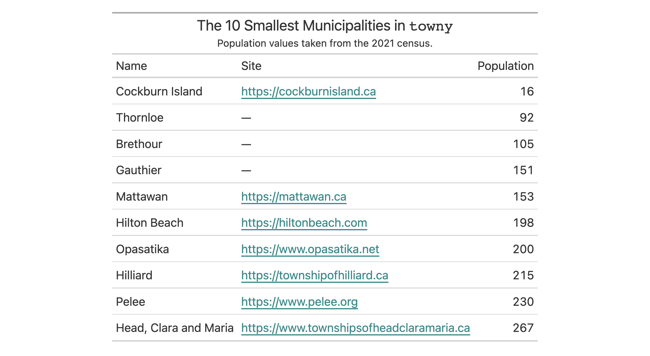
Links can be presented as icons. Let's take a look at an example of this type
of presentation with a table based on the films dataset. The imdb_url
column contains the URL information and in the fmt_url() call, we can use
fontawesome::fa() to specify a label. In this case we elect to use the
"link" icon and we can make some sizing adjustments to the icon here to
ensure the layout looks optimal. We also use cols_merge() to combine
the film's title, its original title (if present), and the link icon.
films |>
dplyr::filter(year == 2021) |>
dplyr::select(
contains("title"), run_time, director, imdb_url
) |>
gt() |>
tab_header(title = "Feature Films in Competition at the 2021 Festival") |>
fmt_url(
columns = imdb_url,
label = fontawesome::fa(
name = "link",
height = "0.75em",
vertical_align = "0em"
),
color = "gray65"
) |>
cols_merge(
columns = c(title, original_title, imdb_url),
pattern = "{1}<< ({2})>> {3}"
) |>
cols_label(
title = "Film",
run_time = "Length",
director = "Director(s)",
) |>
tab_options(heading.title.font.size = px(26)) |>
opt_vertical_padding(scale = 0.4) |>
opt_horizontal_padding(scale = 2) |>
opt_align_table_header(align = "left")

Function ID
3-22
Function Introduced
v0.9.0 (Mar 31, 2023)
See Also
Other data formatting functions:
data_color(),
fmt(),
fmt_auto(),
fmt_bins(),
fmt_bytes(),
fmt_chem(),
fmt_country(),
fmt_currency(),
fmt_date(),
fmt_datetime(),
fmt_duration(),
fmt_email(),
fmt_engineering(),
fmt_flag(),
fmt_fraction(),
fmt_icon(),
fmt_image(),
fmt_index(),
fmt_integer(),
fmt_markdown(),
fmt_number(),
fmt_number_si(),
fmt_partsper(),
fmt_passthrough(),
fmt_percent(),
fmt_roman(),
fmt_scientific(),
fmt_spelled_num(),
fmt_tf(),
fmt_time(),
fmt_units(),
sub_large_vals(),
sub_missing(),
sub_small_vals(),
sub_values(),
sub_zero()
Formatting functions
Description
All formatting functions in gt are quite consistent. All functions that start
with the common fmt_*() prefix have the following points in common
Details
Let's use the exibble data for this.
Examples
gt_tbl <- gt(exibble) # # They all have `columns` and `rows` to specify target cells and default to # styling all compatible cells. # # By default, they apply styling to all compatible columns. # Will style all numeric columns gt_tbl |> fmt_number() # will style the time column gt_tbl |> fmt_time(columns = time) # Will style nothing since is only compatible with logical values gt_tbl |> fmt_tf() # # Their order has importance as the last styling will have priority. # # Will style all numeric columns as integer # fmt_number() will have no effect gt_tbl |> fmt_number() |> fmt_integer() # # Therefore, to apply different styling, it is important to specify columns or rows. # # Will style all numeric columns as number and as currency the currency column. # fmt_number() will have no effect gt_tbl |> fmt_number() |> fmt_integer(currency)gt_tbl <- gt(exibble) # # They all have `columns` and `rows` to specify target cells and default to # styling all compatible cells. # # By default, they apply styling to all compatible columns. # Will style all numeric columns gt_tbl |> fmt_number() # will style the time column gt_tbl |> fmt_time(columns = time) # Will style nothing since is only compatible with logical values gt_tbl |> fmt_tf() # # Their order has importance as the last styling will have priority. # # Will style all numeric columns as integer # fmt_number() will have no effect gt_tbl |> fmt_number() |> fmt_integer() # # Therefore, to apply different styling, it is important to specify columns or rows. # # Will style all numeric columns as number and as currency the currency column. # fmt_number() will have no effect gt_tbl |> fmt_number() |> fmt_integer(currency)
Reference a column of values for certain parameters
Description
It can be useful to obtain parameter values from a column in a
gt for functions that operate on the table body and stub cells. For
example, you might want to indent row labels in the stub. You could call
tab_stub_indent() and indent different rows to various indentation levels.
However, each level of indentation applied necessitates a new call of that
function. To make this better, we can use indentation values available in a
table column via the from_column() helper function. For the
tab_stub_indent() case, you'd invoke this helper at the indent argument
and specify the column that has the values.
Usage
from_column(column, na_value = NULL, fn = NULL)from_column(column, na_value = NULL, fn = NULL)
Arguments
column |
Column name
A single column name in quotation marks. Values will be extracted from this column and provided to compatible arguments. |
na_value |
Default replacement for
A single value to replace any |
fn |
Function to apply
If a function is provided here, any values extracted from the table
|
Value
A list object of class gt_column.
Functions that allow the use of the from_column() helper
Only certain functions (and furthermore a subset of arguments within each)
support the use of from_column() for accessing varying parameter values.
These functions are:
Within help documents for each of these functions you'll find the
Compatibility of arguments with the from_column() helper function section
and sections like these describe which arguments support the use of
from_column().
Examples
from_column() can be used in a variety of formatting functions so that
values for common options don't have to be static, they can change in every
row (so long as you have a column of compatible option values). Here's an
example where we have a table of repeating numeric values along with a column
of currency codes. We can format the numbers to currencies with
fmt_currency() and use from_column() to reference the column of currency
codes, giving us values that are each formatted as having a different
currency.
dplyr::tibble(
amount = rep(30.75, 6),
curr = c("USD", "EUR", "GBP", "CAD", "AUD", "JPY"),
) |>
gt() |>
fmt_currency(currency = from_column(column = "curr"))

Let's summarize the gtcars dataset to get a set of rankings of car
manufacturer by country of origin. The n column represents the number of
cars a manufacturer has within this dataset and we can use that column as a
way to size the text. We do that in the tab_style() call; the
from_column() function is used within the cell_text() statement to
fashion different font sizes from that n column. This is done in
conjunction with the fn argument of from_column(), which helps to tweak
the values in n to get a useful range of font sizes.
gtcars |>
dplyr::count(mfr, ctry_origin) |>
dplyr::arrange(ctry_origin) |>
gt(groupname_col = "ctry_origin") |>
tab_style(
style = cell_text(
size = from_column(
column = "n",
fn = function(x) paste0(5 + (x * 3), "px")
)
),
locations = cells_body()
) |>
tab_style(
style = cell_text(align = "center"),
locations = cells_row_groups()
) |>
cols_hide(columns = n) |>
tab_options(column_labels.hidden = TRUE) |>
opt_all_caps() |>
opt_vertical_padding(scale = 0.25) |>
cols_align(align = "center", columns = mfr)

Function ID
8-5
Function Introduced
v0.10.0 (October 7, 2023)
See Also
Other helper functions:
adjust_luminance(),
cell_borders(),
cell_fill(),
cell_text(),
currency(),
default_fonts(),
escape_latex(),
google_font(),
gt_latex_dependencies(),
html(),
latex(),
md(),
nanoplot_options(),
pct(),
px(),
random_id(),
row_group(),
stub(),
system_fonts(),
unit_conversion()
Helper function for adding a ggplot
Description
We can add a ggplot2 plot inside of a table with the help of the
ggplot_image() function. The function provides a convenient way to generate
an HTML fragment with a ggplot object. Because this function is currently
HTML-based, it is only useful for HTML table output. To use this function
inside of data cells, it is recommended that text_transform() is used.
With that function, we can specify which data cells to target and then
include a call to ggplot_image() within the required user-defined function
(for the fn argument). If we want to include a plot in other places (e.g.,
in the header, within footnote text, etc.) we need to use ggplot_image()
within the html() helper function.
By itself, the function creates an HTML image tag with an image URI embedded
within (a 100 dpi PNG). We can easily experiment with any ggplot2 plot
object, and using it within ggplot_image(plot_object = <plot object>
evaluates to:
<img src=<data URI> style=\"height:100px;\">
where a height of 100px is a default height chosen to work well within the
heights of most table rows. There is the option to modify the aspect ratio of
the plot (the default aspect_ratio is 1.0) and this is useful for
elongating any given plot to fit better within the table construct.
Usage
ggplot_image(plot_object, height = 100, aspect_ratio = 1)ggplot_image(plot_object, height = 100, aspect_ratio = 1)
Arguments
plot_object |
A ggplot plot object
A |
height |
Height of image
The absolute height of the output image in the table cell (in |
aspect_ratio |
The final aspect ratio of plot
This is the plot's final aspect ratio. Where the height of the plot is
fixed using the |
Value
A character object with an HTML fragment that can be placed inside of a cell.
Examples
Create a ggplot plot.
library(ggplot2)
plot_object <-
ggplot(
data = gtcars,
aes(x = hp, y = trq, size = msrp)
) +
geom_point(color = "blue") +
theme(legend.position = "none")
Create a tibble that contains two cells (where one is a placeholder for an
image), then, create a gt table. Use the text_transform() function to
insert the plot using by calling ggplot_object() within the user- defined
function.
dplyr::tibble(
text = "Here is a ggplot:",
ggplot = NA
) |>
gt() |>
text_transform(
locations = cells_body(columns = ggplot),
fn = function(x) {
plot_object |>
ggplot_image(height = px(200))
}
)

Function ID
9-3
Function Introduced
v0.2.0.5 (March 31, 2020)
See Also
Other image addition functions:
local_image(),
test_image(),
web_image()
Weather conditions in Gibraltar, May 2023
Description
The gibraltar dataset has meteorological data for the Gibraltar Airport
Station from May 1 to May 31, 2023. Gibraltar is a British Overseas Territory
and city located at the southern end of the Iberian Peninsula, on the Bay of
Gibraltar. This weather station is located at the airport (GIB), where it's
at an elevation of 5 meters above mean sea level (AMSL).
Usage
gibraltargibraltar
Format
A tibble with 1,431 rows and 10 variables:
- date, time
-
The date and time of the observation.
- temp, dew_point
-
The air temperature and dew point values, both in degrees Celsius.
- humidity
-
The relative humidity as a value between
0and1 - wind_dir, wind_speed, wind_gust
-
Observations related to wind. The wind direction is given as the typical 'blowing from' value, simplified to one of 16 compass directions. The wind speed is provided in units of meters per second. If there was a measurable wind gust, the maximum gust speed is recorded as m/s values (otherwise the value is
0). - pressure
-
The atmospheric pressure in hectopascals (hPa).
- condition
-
The weather condition.
Dataset ID and Badge
DATA-11

Dataset Introduced
v0.11.0 (July 9, 2024)
See Also
Other datasets:
constants,
countrypops,
exibble,
films,
gtcars,
illness,
metro,
nuclides,
peeps,
photolysis,
pizzaplace,
reactions,
rx_addv,
rx_adsl,
sp500,
sza,
towny
Examples
dplyr::glimpse(gibraltar)dplyr::glimpse(gibraltar)
Helper function for specifying a font from the Google Fonts service
Description
google_font() can be used wherever a font name should be specified. There
are two instances where this helper can be used: the name argument in
opt_table_font() (for setting a table font) and in that of cell_text()
(used with tab_style()). To get a helpful listing of fonts that work well
in tables, call info_google_fonts().
Usage
google_font(name)google_font(name)
Arguments
name |
Google Font name
The complete name of a font available in Google Fonts. |
Value
An object of class font_css.
Examples
Use the exibble dataset to create a gt table of two columns and eight
rows. We'll replace missing values with em dashes using sub_missing().
For text in the time column, we will use the font called "IBM Plex Mono"
which is available in Google Fonts. This is defined inside the
google_font() call, itself part of a vector that includes fonts returned by
default_fonts() (those fonts will serve as fallbacks just in case the font
supplied by Google Fonts is not accessible). In terms of placement, all of
this is given to the font argument of cell_text() which is itself given
to the style argument of tab_style().
exibble |>
dplyr::select(char, time) |>
gt() |>
sub_missing() |>
tab_style(
style = cell_text(
font = c(
google_font(name = "IBM Plex Mono"),
default_fonts()
)
),
locations = cells_body(columns = time)
)

We can use a subset of the sp500 dataset to create a small gt table.
With fmt_currency(), we can display a dollar sign for the first row of the
monetary values. Then, we'll set a larger font size for the table and opt to
use the "Merriweather" font by calling google_font() within
opt_table_font(). In cases where that font may not materialize, we include
two font fallbacks: "Cochin" and the catchall "Serif" group.
sp500 |>
dplyr::slice(1:10) |>
dplyr::select(-volume, -adj_close) |>
gt() |>
fmt_currency(
rows = 1,
currency = "USD",
use_seps = FALSE
) |>
tab_options(table.font.size = px(20)) |>
opt_table_font(
font = list(
google_font(name = "Merriweather"),
"Cochin", "Serif"
)
)
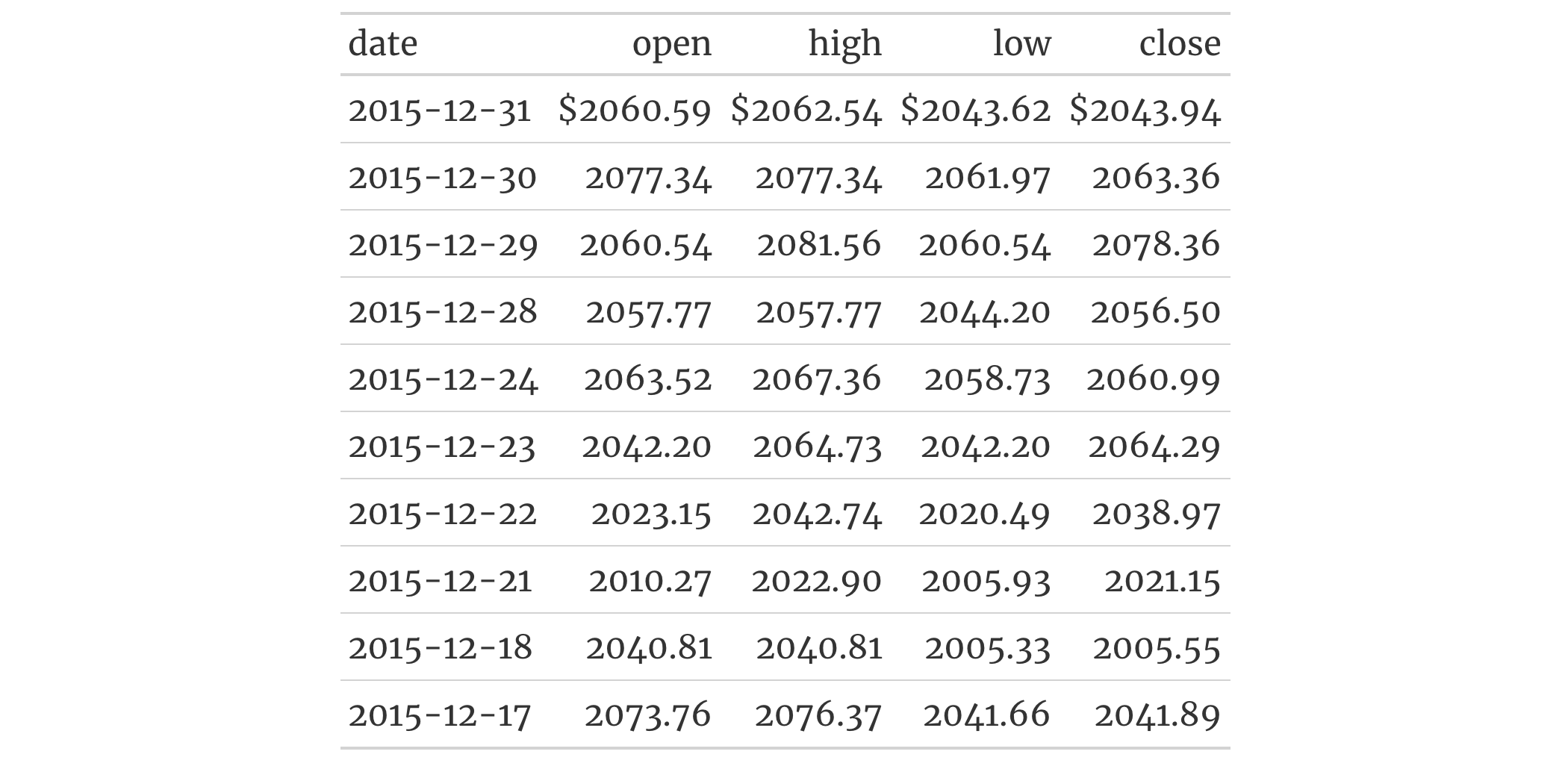
Function ID
8-31
Function Introduced
v0.2.2 (August 5, 2020)
See Also
Other helper functions:
adjust_luminance(),
cell_borders(),
cell_fill(),
cell_text(),
currency(),
default_fonts(),
escape_latex(),
from_column(),
gt_latex_dependencies(),
html(),
latex(),
md(),
nanoplot_options(),
pct(),
px(),
random_id(),
row_group(),
stub(),
system_fonts(),
unit_conversion()
Add grand summary rows using aggregation functions
Description
Add grand summary rows by using the table data and any suitable aggregation
functions. With grand summary rows, all of the available data in the gt
table is incorporated (regardless of whether some of the data are part of row
groups). Multiple grand summary rows can be added via expressions given to
fns. You can selectively format the values in the resulting grand summary
cells by use of formatting expressions in fmt.
Usage
grand_summary_rows( data, columns = everything(), fns = NULL, fmt = NULL, side = c("bottom", "top"), missing_text = "---", formatter = NULL, ... )grand_summary_rows( data, columns = everything(), fns = NULL, fmt = NULL, side = c("bottom", "top"), missing_text = "---", formatter = NULL, ... )
Arguments
data |
The gt table data object
This is the gt table object that is commonly created through use of the
|
columns |
Columns to target
The columns for which the summaries should be calculated. Can either
be a series of column names provided in |
fns |
Aggregation Expressions
Functions used for aggregations. This can include base functions like
|
fmt |
Formatting expressions
Formatting expressions in formula form. The RHS of |
side |
Side used for placement of grand summary rows
Should the grand summary rows be placed at the |
missing_text |
Replacement text for
The text to be used in place of |
formatter |
Deprecated Formatting function
Deprecated, please use |
... |
Deprecated Formatting arguments
Deprecated (along with |
Value
An object of class gt_tbl.
Using columns to target column data for aggregation
Targeting of column data for which aggregates should be generated is done
through the columns argument. We can declare column names in c() (with
bare column names or names in quotes) or we can use
tidyselect-style expressions. This can be as basic as supplying a select
helper like starts_with(), or, providing a more complex incantation like
where(~ is.numeric(.x) & max(.x, na.rm = TRUE) > 1E6)
which targets numeric columns that have a maximum value greater than
1,000,000 (excluding any NAs from consideration).
By default all columns are selected (with the everything() default). This
default may be not what's needed unless all columns can undergo useful
aggregation by expressions supplied in fns.
Aggregation expressions for fns
There are a number of ways to express how an aggregation should work for
each summary row. In addition to that, we have the ability to pass important
information such as the summary row ID value and its label (the former
necessary for targeting within tab_style() or tab_footnote() and the
latter used for display in the rendered table). Here are a number of
instructive examples for how to supply such expressions.
Double-sided formula with everything supplied
We can be explicit and provide a double-sided formula (in the form
<LHS> ~ <RHS>) that expresses everything about a summary row. That is, it
has an aggregation expression (where . represents the data in the
focused column). Here's an example:
list(id = "minimum", label = "min") ~ min(., na.rm = TRUE)
The left side (the list) contains named elements that identify the id and
label for the summary row. The right side has an expression for obtaining
a minimum value (dropping NA values in the calculation).
The list() can be replaced with c() but the advantage of a list is
allowing the use of the md() and html() helper functions. The above
example can be written as:
list(id = "minimum", label = md("**Minimum**")) ~ min(., na.rm = TRUE)
and we can have that label value interpreted as Markdown text.
Function names in quotes
With fns = "min" we get the equivalent of the fuller expression:
list(id = "min", label = "min") ~ min(., na.rm = TRUE)
For sake of convenience, common aggregation functions with the na.rm
argument will be rewritten with the na.rm = TRUE option. These functions
are: "min", "max", "mean", "median", "sd", and "sum".
Should you need to specify multiple aggregation functions in this way (giving
you multiple summary rows), use c() or list().
RHS formula expressions
With fns = ~ min(.) or fns = list(~ min(.)), gt will use the function
name as the id and label. The expansion of this shorthand to full form
looks like this:
list(id = "min", label = "min") ~ min(.)
The RHS expression is kept as written and the name portion is both the id
and the label.
Named vector or list with RHS formula expression
Using fns = c(minimum = ~ min(.)) or fns = list(minimum = ~ min(.))
expands to this:
list(id = "minimum", label = "minimum") ~ min(.)
Unnamed vector or list with RHS formula expression
With fns = c("minimum", "min") ~ min(.) or
fns = list("minimum", "min") ~ min(.) the LHS contains the label and id
values and, importantly, the order is label first and id second. This can
be rewritten as:
list(id = "min", label = "minimum") ~ min(.)
If the vector or list is partially named, gt has enough to go on to
disambiguate the unnamed element. So with
fns = c("minimum", label = "min") ~ min(.), "min" is indeed the label
and "minimum" is taken as the id value.
A fully named list with three specific elements
We can avoid using a formula if we are satisfied with the default options of
a function (except some of those functions with the na.rm options, see
above). Instead, a list with the named elements id, label, and fn could
be used. It can look like this:
fns = list(id = "mean_id", label = "average", fn = "mean")
which translates to
list(id = "mean_id", label = "average") ~ mean(., na.rm = TRUE)
Formatting expressions for fmt
Given that we are generating new data in a table, we might also want to
take the opportunity to format those new values right away. We can do this
in the fmt argument, either with a single expression or a number of them
in a list.
We can supply a one-sided (RHS only) expression to fmt, and, several can
be provided in a list. The expression uses a formatting function (e.g.,
fmt_number(), fmt_currency(), etc.) and it must contain an initial .
that stands for the data object. If performing numeric formatting on all
columns in the new grand summary rows, it might look something like this:
fmt = ~ fmt_number(., decimals = 1, use_seps = FALSE)
We can use the columns and rows arguments that are available in every
formatting function. This allows us to format only a subset of columns or
rows. Summary rows can be targeted by using their ID values and these are
settable within expressions given to fns (see the Aggregation expressions
for fns section for details on this). Here's an example with hypothetical
column and row names:
fmt = ~ fmt_number(., columns = num, rows = "mean", decimals = 3)
Extraction of summary rows
Should we need to obtain the summary data for external purposes,
extract_summary() can be used with a gt_tbl object where summary rows
were added via grand_summary_rows() or summary_rows().
Examples
Use a modified version of the sp500 dataset to create a gt table with
row groups and row labels. Create the grand summary rows min, max, and
avg for the table with grand_summary_rows().
sp500 |>
dplyr::filter(date >= "2015-01-05" & date <= "2015-01-16") |>
dplyr::arrange(date) |>
dplyr::mutate(week = paste0("W", strftime(date, format = "%V"))) |>
dplyr::select(-adj_close, -volume) |>
gt(
rowname_col = "date",
groupname_col = "week"
) |>
grand_summary_rows(
columns = c(open, high, low, close),
fns = list(
min ~ min(.),
max ~ max(.),
avg ~ mean(.)
),
fmt = ~ fmt_number(., use_seps = FALSE)
)
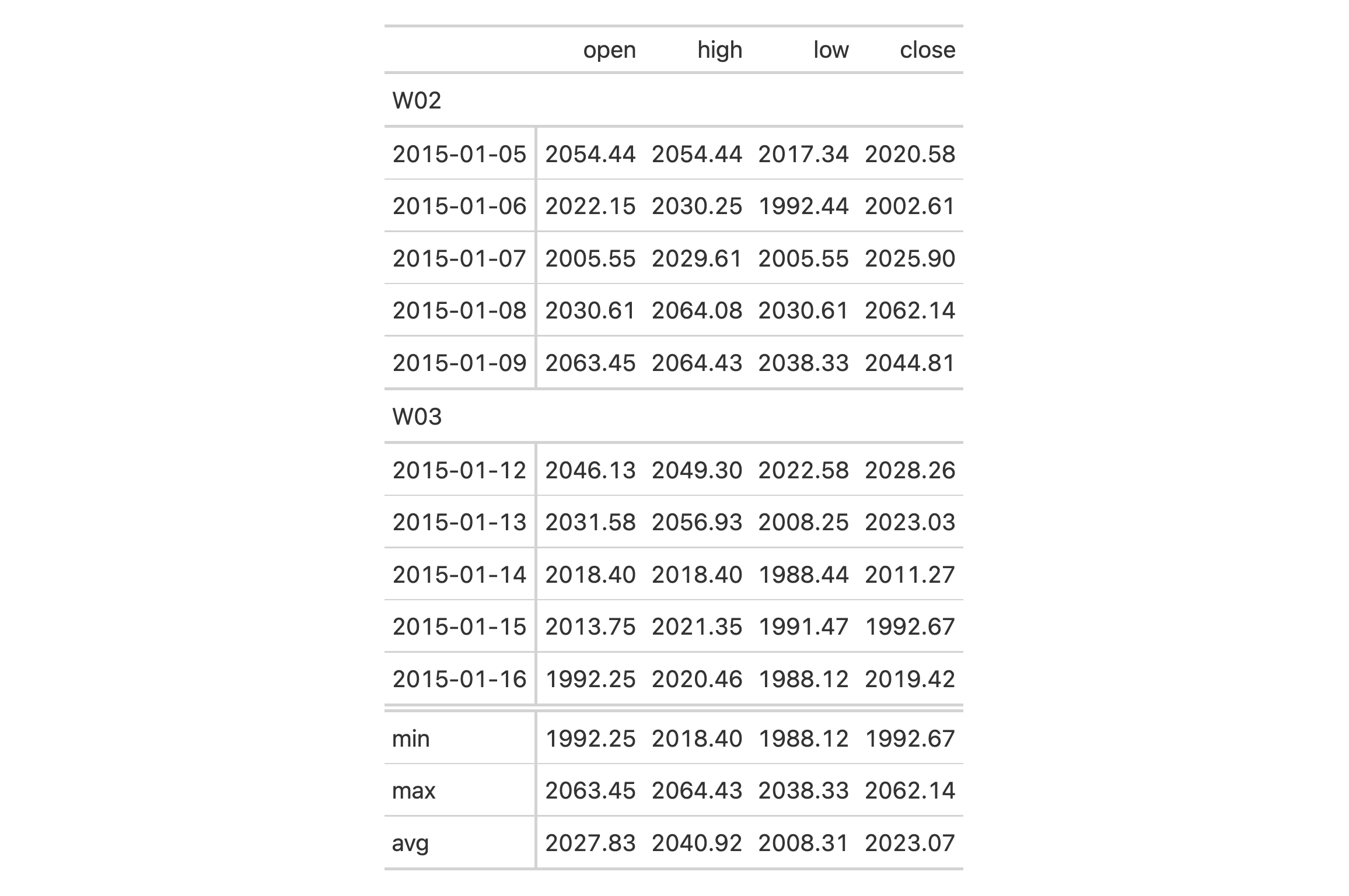
Let's take the countrypops dataset and process that a bit before handing
it off to gt. We can create a single grand summary row with totals that
appears at the top of the table body (with side = "top"). We can define the
aggregation with a list that contains parameters for the grand summary row
label ("TOTALS"), the ID value of that row ("totals"), and the
aggregation function (expressed as "sum", which gt recognizes as the
sum() function). Finally, we'll add a background fill to the grand summary
row with tab_style().
countrypops |>
dplyr::filter(country_code_2 %in% c("BE", "NL", "LU")) |>
dplyr::filter(year %% 10 == 0) |>
dplyr::select(country_name, year, population) |>
tidyr::pivot_wider(names_from = year, values_from = population) |>
gt(rowname_col = "country_name") |>
tab_header(title = "Populations of the Benelux Countries") |>
tab_spanner(columns = everything(), label = "Year") |>
fmt_integer() |>
grand_summary_rows(
fns = list(label = "TOTALS", id = "totals", fn = "sum"),
fmt = ~ fmt_integer(.),
side = "top"
) |>
tab_style(
locations = cells_grand_summary(),
style = cell_fill(color = "lightblue" |> adjust_luminance(steps = +1))
)

Function ID
6-2
Function Introduced
v0.2.0.5 (March 31, 2020)
See Also
Other row addition/modification functions:
row_group_order(),
row_order(),
rows_add(),
rows_hide(),
rows_unhide(),
summary_columns(),
summary_rows()
Add one or more gt tables to a gt_group container object
Description
Should you have a gt_group object, created through use of the gt_group()
function, you might want to add more gt tables to that container. While
it's common to generate a gt_group object with a collection of gt_tbl
objects, one can also create an 'empty' gt_group object. Whatever your
workflow might be, the grp_add() function makes it possible to flexibly
add one or more new gt tables, returning a refreshed gt_group object.
Usage
grp_add(.data, ..., .list = list2(...), .before = NULL, .after = NULL)grp_add(.data, ..., .list = list2(...), .before = NULL, .after = NULL)
Arguments
.data |
The gt table group object
This is a |
... |
One or more gt table objects
One or more gt table ( |
.list |
Alternative to
Allows for the use of a list as an input alternative to |
.before, .after
|
Table used as anchor
A single index for either |
Value
An object of class gt_group.
Function ID
14-4
Function Introduced
v0.9.0 (Mar 31, 2023)
See Also
Other table group functions:
grp_clone(),
grp_options(),
grp_pull(),
grp_replace(),
grp_rm(),
gt_group(),
gt_split()
Clone one or more gt tables in a gt_group container object
Description
Should you have a gt_group object, created through use of the gt_group()
function, you may in certain circumstances want to create replicas of
gt_tbl objects in that collection. This can be done with the grp_clone()
function and the placement of the cloned gt tables can be controlled with
either the before or after arguments.
Usage
grp_clone(data, which = NULL, before = NULL, after = NULL)grp_clone(data, which = NULL, before = NULL, after = NULL)
Arguments
data |
The gt table group object
This is a |
which |
The tables to clone
A vector of index values denoting which gt tables should be cloned
inside of the |
before, after
|
Table used as anchor
A single index for either |
Value
An object of class gt_group.
Function ID
14-5
Function Introduced
v0.9.0 (Mar 31, 2023)
See Also
Other table group functions:
grp_add(),
grp_options(),
grp_pull(),
grp_replace(),
grp_rm(),
gt_group(),
gt_split()
Modify table options for all tables within a gt_group object
Description
Modify the options for a collection of gt tables in a gt_group object.
These options are named by the components, the subcomponents, and the
element that can adjusted.
Usage
grp_options( data, table.width = NULL, table.layout = NULL, table.align = NULL, table.margin.left = NULL, table.margin.right = NULL, table.background.color = NULL, table.additional_css = NULL, table.font.names = NULL, table.font.size = NULL, table.font.weight = NULL, table.font.style = NULL, table.font.color = NULL, table.font.color.light = NULL, table.border.top.style = NULL, table.border.top.width = NULL, table.border.top.color = NULL, table.border.right.style = NULL, table.border.right.width = NULL, table.border.right.color = NULL, table.border.bottom.style = NULL, table.border.bottom.width = NULL, table.border.bottom.color = NULL, table.border.left.style = NULL, table.border.left.width = NULL, table.border.left.color = NULL, heading.background.color = NULL, heading.align = NULL, heading.title.font.size = NULL, heading.title.font.weight = NULL, heading.subtitle.font.size = NULL, heading.subtitle.font.weight = NULL, heading.padding = NULL, heading.padding.horizontal = NULL, heading.border.bottom.style = NULL, heading.border.bottom.width = NULL, heading.border.bottom.color = NULL, heading.border.lr.style = NULL, heading.border.lr.width = NULL, heading.border.lr.color = NULL, column_labels.background.color = NULL, column_labels.font.size = NULL, column_labels.font.weight = NULL, column_labels.text_transform = NULL, column_labels.padding = NULL, column_labels.padding.horizontal = NULL, column_labels.vlines.style = NULL, column_labels.vlines.width = NULL, column_labels.vlines.color = NULL, column_labels.border.top.style = NULL, column_labels.border.top.width = NULL, column_labels.border.top.color = NULL, column_labels.border.bottom.style = NULL, column_labels.border.bottom.width = NULL, column_labels.border.bottom.color = NULL, column_labels.border.lr.style = NULL, column_labels.border.lr.width = NULL, column_labels.border.lr.color = NULL, column_labels.hidden = NULL, column_labels.units_pattern = NULL, row_group.background.color = NULL, row_group.font.size = NULL, row_group.font.weight = NULL, row_group.text_transform = NULL, row_group.padding = NULL, row_group.padding.horizontal = NULL, row_group.border.top.style = NULL, row_group.border.top.width = NULL, row_group.border.top.color = NULL, row_group.border.bottom.style = NULL, row_group.border.bottom.width = NULL, row_group.border.bottom.color = NULL, row_group.border.left.style = NULL, row_group.border.left.width = NULL, row_group.border.left.color = NULL, row_group.border.right.style = NULL, row_group.border.right.width = NULL, row_group.border.right.color = NULL, row_group.default_label = NULL, row_group.as_column = NULL, table_body.hlines.style = NULL, table_body.hlines.width = NULL, table_body.hlines.color = NULL, table_body.vlines.style = NULL, table_body.vlines.width = NULL, table_body.vlines.color = NULL, table_body.border.top.style = NULL, table_body.border.top.width = NULL, table_body.border.top.color = NULL, table_body.border.bottom.style = NULL, table_body.border.bottom.width = NULL, table_body.border.bottom.color = NULL, stub.background.color = NULL, stub.font.size = NULL, stub.font.weight = NULL, stub.text_transform = NULL, stub.border.style = NULL, stub.border.width = NULL, stub.border.color = NULL, stub.indent_length = NULL, stub_row_group.font.size = NULL, stub_row_group.font.weight = NULL, stub_row_group.text_transform = NULL, stub_row_group.border.style = NULL, stub_row_group.border.width = NULL, stub_row_group.border.color = NULL, data_row.padding = NULL, data_row.padding.horizontal = NULL, summary_row.background.color = NULL, summary_row.text_transform = NULL, summary_row.padding = NULL, summary_row.padding.horizontal = NULL, summary_row.border.style = NULL, summary_row.border.width = NULL, summary_row.border.color = NULL, grand_summary_row.background.color = NULL, grand_summary_row.text_transform = NULL, grand_summary_row.padding = NULL, grand_summary_row.padding.horizontal = NULL, grand_summary_row.border.style = NULL, grand_summary_row.border.width = NULL, grand_summary_row.border.color = NULL, footnotes.background.color = NULL, footnotes.font.size = NULL, footnotes.padding = NULL, footnotes.padding.horizontal = NULL, footnotes.border.bottom.style = NULL, footnotes.border.bottom.width = NULL, footnotes.border.bottom.color = NULL, footnotes.border.lr.style = NULL, footnotes.border.lr.width = NULL, footnotes.border.lr.color = NULL, footnotes.marks = NULL, footnotes.spec_ref = NULL, footnotes.spec_ftr = NULL, footnotes.multiline = NULL, footnotes.sep = NULL, source_notes.background.color = NULL, source_notes.font.size = NULL, source_notes.padding = NULL, source_notes.padding.horizontal = NULL, source_notes.border.bottom.style = NULL, source_notes.border.bottom.width = NULL, source_notes.border.bottom.color = NULL, source_notes.border.lr.style = NULL, source_notes.border.lr.width = NULL, source_notes.border.lr.color = NULL, source_notes.multiline = NULL, source_notes.sep = NULL, row.striping.background_color = NULL, row.striping.include_stub = NULL, row.striping.include_table_body = NULL, container.width = NULL, container.height = NULL, container.padding.x = NULL, container.padding.y = NULL, container.overflow.x = NULL, container.overflow.y = NULL, ihtml.active = NULL, ihtml.use_pagination = NULL, ihtml.use_pagination_info = NULL, ihtml.use_sorting = NULL, ihtml.use_search = NULL, ihtml.use_filters = NULL, ihtml.use_resizers = NULL, ihtml.use_highlight = NULL, ihtml.use_compact_mode = NULL, ihtml.use_text_wrapping = NULL, ihtml.use_page_size_select = NULL, ihtml.page_size_default = NULL, ihtml.page_size_values = NULL, ihtml.pagination_type = NULL, page.orientation = NULL, page.numbering = NULL, page.header.use_tbl_headings = NULL, page.footer.use_tbl_notes = NULL, page.width = NULL, page.height = NULL, page.margin.left = NULL, page.margin.right = NULL, page.margin.top = NULL, page.margin.bottom = NULL, page.header.height = NULL, page.footer.height = NULL )grp_options( data, table.width = NULL, table.layout = NULL, table.align = NULL, table.margin.left = NULL, table.margin.right = NULL, table.background.color = NULL, table.additional_css = NULL, table.font.names = NULL, table.font.size = NULL, table.font.weight = NULL, table.font.style = NULL, table.font.color = NULL, table.font.color.light = NULL, table.border.top.style = NULL, table.border.top.width = NULL, table.border.top.color = NULL, table.border.right.style = NULL, table.border.right.width = NULL, table.border.right.color = NULL, table.border.bottom.style = NULL, table.border.bottom.width = NULL, table.border.bottom.color = NULL, table.border.left.style = NULL, table.border.left.width = NULL, table.border.left.color = NULL, heading.background.color = NULL, heading.align = NULL, heading.title.font.size = NULL, heading.title.font.weight = NULL, heading.subtitle.font.size = NULL, heading.subtitle.font.weight = NULL, heading.padding = NULL, heading.padding.horizontal = NULL, heading.border.bottom.style = NULL, heading.border.bottom.width = NULL, heading.border.bottom.color = NULL, heading.border.lr.style = NULL, heading.border.lr.width = NULL, heading.border.lr.color = NULL, column_labels.background.color = NULL, column_labels.font.size = NULL, column_labels.font.weight = NULL, column_labels.text_transform = NULL, column_labels.padding = NULL, column_labels.padding.horizontal = NULL, column_labels.vlines.style = NULL, column_labels.vlines.width = NULL, column_labels.vlines.color = NULL, column_labels.border.top.style = NULL, column_labels.border.top.width = NULL, column_labels.border.top.color = NULL, column_labels.border.bottom.style = NULL, column_labels.border.bottom.width = NULL, column_labels.border.bottom.color = NULL, column_labels.border.lr.style = NULL, column_labels.border.lr.width = NULL, column_labels.border.lr.color = NULL, column_labels.hidden = NULL, column_labels.units_pattern = NULL, row_group.background.color = NULL, row_group.font.size = NULL, row_group.font.weight = NULL, row_group.text_transform = NULL, row_group.padding = NULL, row_group.padding.horizontal = NULL, row_group.border.top.style = NULL, row_group.border.top.width = NULL, row_group.border.top.color = NULL, row_group.border.bottom.style = NULL, row_group.border.bottom.width = NULL, row_group.border.bottom.color = NULL, row_group.border.left.style = NULL, row_group.border.left.width = NULL, row_group.border.left.color = NULL, row_group.border.right.style = NULL, row_group.border.right.width = NULL, row_group.border.right.color = NULL, row_group.default_label = NULL, row_group.as_column = NULL, table_body.hlines.style = NULL, table_body.hlines.width = NULL, table_body.hlines.color = NULL, table_body.vlines.style = NULL, table_body.vlines.width = NULL, table_body.vlines.color = NULL, table_body.border.top.style = NULL, table_body.border.top.width = NULL, table_body.border.top.color = NULL, table_body.border.bottom.style = NULL, table_body.border.bottom.width = NULL, table_body.border.bottom.color = NULL, stub.background.color = NULL, stub.font.size = NULL, stub.font.weight = NULL, stub.text_transform = NULL, stub.border.style = NULL, stub.border.width = NULL, stub.border.color = NULL, stub.indent_length = NULL, stub_row_group.font.size = NULL, stub_row_group.font.weight = NULL, stub_row_group.text_transform = NULL, stub_row_group.border.style = NULL, stub_row_group.border.width = NULL, stub_row_group.border.color = NULL, data_row.padding = NULL, data_row.padding.horizontal = NULL, summary_row.background.color = NULL, summary_row.text_transform = NULL, summary_row.padding = NULL, summary_row.padding.horizontal = NULL, summary_row.border.style = NULL, summary_row.border.width = NULL, summary_row.border.color = NULL, grand_summary_row.background.color = NULL, grand_summary_row.text_transform = NULL, grand_summary_row.padding = NULL, grand_summary_row.padding.horizontal = NULL, grand_summary_row.border.style = NULL, grand_summary_row.border.width = NULL, grand_summary_row.border.color = NULL, footnotes.background.color = NULL, footnotes.font.size = NULL, footnotes.padding = NULL, footnotes.padding.horizontal = NULL, footnotes.border.bottom.style = NULL, footnotes.border.bottom.width = NULL, footnotes.border.bottom.color = NULL, footnotes.border.lr.style = NULL, footnotes.border.lr.width = NULL, footnotes.border.lr.color = NULL, footnotes.marks = NULL, footnotes.spec_ref = NULL, footnotes.spec_ftr = NULL, footnotes.multiline = NULL, footnotes.sep = NULL, source_notes.background.color = NULL, source_notes.font.size = NULL, source_notes.padding = NULL, source_notes.padding.horizontal = NULL, source_notes.border.bottom.style = NULL, source_notes.border.bottom.width = NULL, source_notes.border.bottom.color = NULL, source_notes.border.lr.style = NULL, source_notes.border.lr.width = NULL, source_notes.border.lr.color = NULL, source_notes.multiline = NULL, source_notes.sep = NULL, row.striping.background_color = NULL, row.striping.include_stub = NULL, row.striping.include_table_body = NULL, container.width = NULL, container.height = NULL, container.padding.x = NULL, container.padding.y = NULL, container.overflow.x = NULL, container.overflow.y = NULL, ihtml.active = NULL, ihtml.use_pagination = NULL, ihtml.use_pagination_info = NULL, ihtml.use_sorting = NULL, ihtml.use_search = NULL, ihtml.use_filters = NULL, ihtml.use_resizers = NULL, ihtml.use_highlight = NULL, ihtml.use_compact_mode = NULL, ihtml.use_text_wrapping = NULL, ihtml.use_page_size_select = NULL, ihtml.page_size_default = NULL, ihtml.page_size_values = NULL, ihtml.pagination_type = NULL, page.orientation = NULL, page.numbering = NULL, page.header.use_tbl_headings = NULL, page.footer.use_tbl_notes = NULL, page.width = NULL, page.height = NULL, page.margin.left = NULL, page.margin.right = NULL, page.margin.top = NULL, page.margin.bottom = NULL, page.header.height = NULL, page.footer.height = NULL )
Arguments
data |
The gt table group object
This is a |
table.width |
Table width The table width can be specified as a single-length character with units of
pixels or as a percentage. If provided as a single-length numeric vector,
it is assumed that the value is given in units of pixels. The |
table.layout |
The table-layout property This is the value for the |
table.align |
Horizontal alignment of table The |
table.margin.left, table.margin.right
|
Left and right table margins The size of the margins on the left and right of the table within the
container can be set with |
table.background.color, heading.background.color, column_labels.background.color, row_group.background.color, stub.background.color, summary_row.background.color, grand_summary_row.background.color, footnotes.background.color, source_notes.background.color
|
Background colors These options govern background colors for the parent element |
table.additional_css |
Additional CSS The |
table.font.names |
Default table fonts The names of the fonts used for the table can be supplied through
|
table.font.size, heading.title.font.size, heading.subtitle.font.size, column_labels.font.size, row_group.font.size, stub.font.size, footnotes.font.size, source_notes.font.size
|
Table font sizes The font sizes for the parent text element |
table.font.weight, heading.title.font.weight, heading.subtitle.font.weight, column_labels.font.weight, row_group.font.weight, stub.font.weight
|
Table font weights The font weights of the table, |
table.font.style |
Default table font style This is the default font style for the table. Can be one of either
|
table.font.color, table.font.color.light
|
Default dark and light text for the table These options define text colors used throughout the table. There are two
variants: |
table.border.top.style, table.border.top.width, table.border.top.color, table.border.right.style, table.border.right.width, table.border.right.color, table.border.bottom.style, table.border.bottom.width, table.border.bottom.color, table.border.left.style, table.border.left.width, table.border.left.color
|
Top border properties The style, width, and color properties of the table's absolute top and absolute bottom borders. |
heading.align |
Horizontal alignment in the table header Controls the horizontal alignment of the heading title and subtitle. We can
either use |
heading.padding, column_labels.padding, data_row.padding, row_group.padding, summary_row.padding, grand_summary_row.padding, footnotes.padding, source_notes.padding
|
Vertical padding throughout the table The amount of vertical padding to incorporate in the |
heading.padding.horizontal, column_labels.padding.horizontal, data_row.padding.horizontal, row_group.padding.horizontal, summary_row.padding.horizontal, grand_summary_row.padding.horizontal, footnotes.padding.horizontal, source_notes.padding.horizontal
|
Horizontal padding throughout the table The amount of horizontal padding to incorporate in the |
heading.border.bottom.style, heading.border.bottom.width, heading.border.bottom.color
|
Properties of the header's bottom border The style, width, and color properties of the header's bottom border. This
border shares space with that of the |
heading.border.lr.style, heading.border.lr.width, heading.border.lr.color
|
Properties of the header's left and right borders The style, width, and color properties for the left and right borders of
the |
column_labels.text_transform, row_group.text_transform, stub.text_transform, summary_row.text_transform, grand_summary_row.text_transform
|
Text transforms throughout the table Options to apply text transformations to the |
column_labels.vlines.style, column_labels.vlines.width, column_labels.vlines.color
|
Properties of all vertical lines by the column labels The style, width, and color properties for all vertical lines ('vlines')
of the |
column_labels.border.top.style, column_labels.border.top.width, column_labels.border.top.color
|
Properties of the border above the column labels The style, width, and color properties for the top border of the
|
column_labels.border.bottom.style, column_labels.border.bottom.width, column_labels.border.bottom.color
|
Properties of the border below the column labels The style, width, and color properties for the bottom border of the
|
column_labels.border.lr.style, column_labels.border.lr.width, column_labels.border.lr.color
|
Properties of the left and right borders next to the column labels The style, width, and color properties for the left and right borders of
the |
|
Hiding all column labels An option to hide the column labels. If providing |
|
column_labels.units_pattern |
Pattern to combine column labels and units The default pattern for combining column labels with any defined units for
column labels. The pattern is initialized as |
row_group.border.top.style, row_group.border.top.width, row_group.border.top.color, row_group.border.bottom.style, row_group.border.bottom.width, row_group.border.bottom.color, row_group.border.left.style, row_group.border.left.width, row_group.border.left.color, row_group.border.right.style, row_group.border.right.width, row_group.border.right.color
|
Border properties associated with the The style, width, and color properties for all top, bottom, left, and right
borders of the |
row_group.default_label |
The default row group label An option to set a default row group label for any rows not formally placed
in a row group named by |
row_group.as_column |
Structure row groups with a column How should row groups be structured? By default, they are separate rows
that lie above the each of the groups. Setting this to |
table_body.hlines.style, table_body.hlines.width, table_body.hlines.color, table_body.vlines.style, table_body.vlines.width, table_body.vlines.color
|
Properties of all horizontal and vertical lines in the table body The style, width, and color properties for all horizontal lines ('hlines')
and vertical lines ('vlines') in the |
table_body.border.top.style, table_body.border.top.width, table_body.border.top.color, table_body.border.bottom.style, table_body.border.bottom.width, table_body.border.bottom.color
|
Properties of top and bottom borders in the table body The style, width, and color properties for all top and bottom borders of
the |
stub.border.style, stub.border.width, stub.border.color
|
Properties of the vertical border of the table stub The style, width, and color properties for the vertical border of the table stub. |
stub.indent_length |
Width of each indentation The width of each indentation level for row labels in the stub. The
indentation can be set by using |
stub_row_group.font.size, stub_row_group.font.weight, stub_row_group.text_transform, stub_row_group.border.style, stub_row_group.border.width, stub_row_group.border.color
|
Properties of the row group column in the table stub Options for the row group column in the table stub (made possible when
using |
summary_row.border.style, summary_row.border.width, summary_row.border.color
|
Properties of horizontal borders belonging to summary rows The style, width, and color properties for all horizontal borders of the
|
grand_summary_row.border.style, grand_summary_row.border.width, grand_summary_row.border.color
|
Properties of horizontal borders belonging to grand summary rows The style, width, and color properties for the top borders of the
|
footnotes.border.bottom.style, footnotes.border.bottom.width, footnotes.border.bottom.color
|
Properties of the bottom border belonging to the footnotes The style, width, and color properties for the bottom border of the
|
footnotes.border.lr.style, footnotes.border.lr.width, footnotes.border.lr.color
|
Properties of left and right borders belonging to the footnotes The style, width, and color properties for the left and right borders of
the |
footnotes.marks |
Sequence of footnote marks The set of sequential marks used to reference and identify each of the
footnotes (same input as |
footnotes.spec_ref, footnotes.spec_ftr
|
Specifications for formatting of footnote marks Optional specifications for formatting of footnote references
( |
footnotes.multiline, source_notes.multiline
|
Typesetting of multiple footnotes and source notes An option to either put footnotes and source notes in separate lines (the
default, or |
footnotes.sep, source_notes.sep
|
Separator characters between adjacent footnotes and source notes The separating characters between adjacent footnotes and source notes in
their respective footer sections when rendered as a continuous line of text
(when |
source_notes.border.bottom.style, source_notes.border.bottom.width, source_notes.border.bottom.color
|
Properties of the bottom border belonging to the source notes The style, width, and color properties for the bottom border of the
|
source_notes.border.lr.style, source_notes.border.lr.width, source_notes.border.lr.color
|
Properties of left and right borders belonging to the source notes The style, width, and color properties for the left and right borders of
the |
row.striping.background_color |
Background color for row stripes The background color for striped table body rows. A color name or a hexadecimal color code should be provided. |
row.striping.include_stub |
Inclusion of the table stub for row stripes An option for whether to include the stub when striping rows. |
row.striping.include_table_body |
Inclusion of the table body for row stripes An option for whether to include the table body when striping rows. |
container.width, container.height, container.padding.x, container.padding.y
|
Table container dimensions and padding The width and height of the table's container, and, the vertical and
horizontal padding of the table's container. The container width and height
can be specified with units of pixels or as a percentage. The padding is to
be specified as a length with units of pixels. If provided as a numeric
value, it is assumed that the value is given in units of pixels. The |
container.overflow.x, container.overflow.y
|
Table container overflow Options to enable scrolling in the horizontal and vertical directions when
the table content overflows the container dimensions. Using |
ihtml.active |
Display interactive HTML table The option for displaying an interactive version of an HTML table (rather
than an otherwise 'static' table). This enables the use of controls for
pagination, global search, filtering, and sorting. The individual features
are controlled by the other |
ihtml.use_pagination, ihtml.use_pagination_info
|
Use pagination For interactive HTML output, the option for using pagination controls
(below the table body) can be controlled with |
ihtml.use_sorting |
Provide column sorting controls For interactive HTML output, the option to provide controls for sorting
column values. By default, this is |
ihtml.use_search |
Provide a global search field For interactive HTML output, an option that places a search field for
globally filtering rows to the requested content. By default, this is
|
ihtml.use_filters |
Display filtering fields For interactive HTML output, this places search fields below each column
header and allows for filtering by column. By default, this is |
ihtml.use_resizers |
Allow column resizing For interactive HTML output, this allows for interactive resizing of
columns. By default, this is |
ihtml.use_highlight |
Enable row highlighting on hover For interactive HTML output, this highlights individual rows upon hover. By
default, this is |
ihtml.use_compact_mode |
Use compact mode For interactive HTML output, an option to reduce vertical padding and thus
make the table consume less vertical space. By default, this is |
ihtml.use_text_wrapping |
Use text wrapping For interactive HTML output, an option to control text wrapping. By default
( |
ihtml.use_page_size_select, ihtml.page_size_default, ihtml.page_size_values
|
Change page size properties For interactive HTML output, |
ihtml.pagination_type |
Change pagination mode For interactive HTML output and when using pagination, one of three options
for presentation pagination controls. The default is |
page.orientation |
Set RTF page orientation For RTF output, this provides two options for page
orientation: |
page.numbering |
Enable RTF page numbering Within RTF output, should page numbering be displayed? By default, this is
set to |
page.header.use_tbl_headings |
Place table headings in RTF page header If |
page.footer.use_tbl_notes |
Place table footer in RTF page footer If |
page.width, page.height
|
Set RTF page dimensions The page width and height in the standard portrait orientation. This is for
RTF table output and the default values (in inches) are |
page.margin.left, page.margin.right, page.margin.top, page.margin.bottom
|
Set RTF page margins For RTF table output, these options correspond to the left, right, top, and
bottom page margins. The default values for each of these is |
page.header.height, page.footer.height
|
Set RTF page header and footer distances The heights of the page header and footer for RTF table outputs. Default
values for both are |
Value
An object of class gt_group.
Function ID
14-8
Function Introduced
v0.9.0 (Mar 31, 2023)
See Also
Other table group functions:
grp_add(),
grp_clone(),
grp_pull(),
grp_replace(),
grp_rm(),
gt_group(),
gt_split()
Pull out a gt table from a gt_group container object
Description
Should you have a gt_group object, created through use of gt_group(),
you may have a need to extract a gt table from that container.
grp_pull() makes this possible, returning a gt_tbl object. The only thing
you need to provide is the index value for the gt table within the
gt_group object.
Usage
grp_pull(data, which)grp_pull(data, which)
Arguments
data |
The gt table group object
This is a |
which |
The table to pull from the group
A single index value denoting which |
Value
An object of class gt_tbl.
Function ID
14-3
Function Introduced
v0.9.0 (Mar 31, 2023)
See Also
Other table group functions:
grp_add(),
grp_clone(),
grp_options(),
grp_replace(),
grp_rm(),
gt_group(),
gt_split()
Replace one or more gt tables in a gt_group container object
Description
gt_group() can be used to create a container for multiple gt tables.
In some circumstances, you might want to replace a specific gt_tbl object
(or multiple) with a different one. This can be done with grp_replace().
The important thing is that the number of gt tables provided must equal
the number of indices for tables present in the gt_group object.
Usage
grp_replace(.data, ..., .list = list2(...), .which)grp_replace(.data, ..., .list = list2(...), .which)
Arguments
.data |
The gt table group object
This is a |
... |
One or more gt table objects
One or more gt table ( |
.list |
Alternative to
Allows for the use of a list as an input alternative to |
.which |
The tables to replace
A vector of index values denoting which gt tables should be replaced
inside of the |
Value
An object of class gt_group.
Function ID
14-6
Function Introduced
v0.9.0 (Mar 31, 2023)
See Also
Other table group functions:
grp_add(),
grp_clone(),
grp_options(),
grp_pull(),
grp_rm(),
gt_group(),
gt_split()
Remove one or more gt tables from a gt_group container object
Description
A gt_group object, created through use of the gt_group() function, can
hold a multiple of gt tables. However, you might want to delete one or
more gt_tbl objects table from that container. With grp_rm(), this is
possible and safe to perform. What's returned is a gt_group object with the
specified gt_tbl objects gone. The only thing you need to provide is the
index value for the gt table within the gt_group object.
Usage
grp_rm(data, which)grp_rm(data, which)
Arguments
data |
The gt table group object
This is a |
which |
The table to remove from the group
A single index value denoting which |
Value
An object of class gt_group.
Function ID
14-7
Function Introduced
v0.9.0 (Mar 31, 2023)
See Also
Other table group functions:
grp_add(),
grp_clone(),
grp_options(),
grp_pull(),
grp_replace(),
gt_group(),
gt_split()
Create a gt table object
Description
The gt() function creates a gt table object when provided with table
data. Using this function is the first step in a typical gt workflow.
Once we have the gt table object, we can perform styling transformations
before rendering to a display table of various formats.
Usage
gt( data, rowname_col = NULL, groupname_col = dplyr::group_vars(data), omit_na_group = FALSE, process_md = FALSE, caption = NULL, rownames_to_stub = FALSE, row_group_as_column = FALSE, auto_align = TRUE, id = NULL, locale = getOption("gt.locale"), row_group.sep = getOption("gt.row_group.sep", " - ") )gt( data, rowname_col = NULL, groupname_col = dplyr::group_vars(data), omit_na_group = FALSE, process_md = FALSE, caption = NULL, rownames_to_stub = FALSE, row_group_as_column = FALSE, auto_align = TRUE, id = NULL, locale = getOption("gt.locale"), row_group.sep = getOption("gt.row_group.sep", " - ") )
Arguments
data |
Input data table
A |
rowname_col |
Column(s) for row names/labels from
The column name(s) in the input |
groupname_col |
Column for group names/labels from
The column name in the input |
omit_na_group |
Omit rows with NA in
Should rows with |
process_md |
Process Markdown in
Should the contents of the |
caption |
Table caption text
An optional table caption to use for cross-referencing in R Markdown, Quarto, or bookdown. |
rownames_to_stub |
Use data frame row labels in the stub
An option to take rownames from the input |
row_group_as_column |
Mode for displaying row group labels in the stub
An option that alters the display of row group labels. By default this is
|
auto_align |
Automatic alignment of column values and labels
Optionally have column data be aligned depending on the content contained
in each column of the input |
id |
The table ID
By default (with |
locale |
Locale identifier
An optional locale identifier that can be set as the default locale for all
functions that take a |
row_group.sep |
Separator text for multiple row group labels
The separator to use between consecutive group names (a possibility when
providing |
Details
There are a few data ingest options we can consider at this stage. We can
choose to create a table stub containing row labels through the use of the
rowname_col argument. Further to this, stub row groups can be created with
the groupname_col argument. Both arguments take the name of a column in the
input table data. Typically, the data in the groupname_col column will
consist of categorical text whereas the data in the rowname_col column will
contain unique labels (could be unique across the entire table or unique
within the different row groups).
Row groups can also be created by passing a grouped_df to gt() by using
dplyr::group_by() on the table data. In this way, two or more
columns of categorical data can be used to make row groups. The
row_group.sep argument allows for control in how the row group labels will
appear in the display table.
Value
An object of class gt_tbl.
Examples
Let's use the exibble dataset for the next few examples, we'll learn how
to make simple gt tables with the gt() function. The most basic thing
to do is to just use gt() with the dataset as the input.
exibble |> gt()

This dataset has the row and group columns. The former contains unique
values that are ideal for labeling rows, and this often happens in what is
called the 'stub' (a reserved area that serves to label rows). With the
gt() function, we can immediately place the contents of the row column
into the stub column. To do this, we use the rowname_col argument with the
name of the column to use in quotes.
exibble |> gt(rowname_col = "row")

This sets up a table with a stub, the row labels are placed within the stub column, and a vertical dividing line has been placed on the right-hand side.
The group column can be used to divide the rows into discrete groups.
Within that column, we see repetitions of the values grp_a and grp_b.
These serve both as ID values and the initial label for the groups. With the
groupname_col argument in gt(), we can set up the row groups immediately
upon creation of the table.
exibble |>
gt(
rowname_col = "row",
groupname_col = "group"
)

If you'd rather perform the set up of row groups later (i.e., not in the
gt() call), this is possible with tab_row_group() (and row_group_order()
can help with the arrangement of row groups).
One more thing to consider with row groups is their layout. By default, row
group labels reside in separate rows the appear above the group. However,
we can use row_group_as_column = TRUE to put the row group labels within a
secondary column within the table stub.
exibble |>
gt(
rowname_col = "row",
groupname_col = "group",
row_group_as_column = TRUE
)

This could be done later if need be, and using
tab_options(row_group.as_column = TRUE) would be the way to do it outside
of the gt() call.
Some datasets have rownames built in; mtcars famously has the car model
names as the rownames. To use those rownames as row labels in the stub, the
rownames_to_stub = TRUE option will prove to be useful.
head(mtcars, 10) |> gt(rownames_to_stub = TRUE)

By default, values in the body of a gt table (and their column labels)
are automatically aligned. The alignment is governed by the types of values
in a column. If you'd like to disable this form of auto-alignment, the
auto_align = FALSE option can be taken.
exibble |> gt(rowname_col = "row", auto_align = FALSE)

What you'll get from that is center-alignment of all table body values and
all column labels. Note that row labels in the stub are still
left-aligned; and auto_align has no effect on alignment within the table
stub.
However which way you generate the initial gt table object, you can use
it with a huge variety of functions in the package to further customize the
presentation. Formatting body cells is commonly done with the family of
formatting functions (e.g., fmt_number(), fmt_date(), etc.). The package
supports formatting with internationalization ('i18n' features) and so
locale-aware functions come with a locale argument. To avoid having to use
that argument repeatedly, the gt() function has its own locale argument.
Setting a locale in that will make it available globally. Here's an example
of how that works in practice when setting locale = "fr" in gt() and
using formatting functions:
exibble |>
gt(
rowname_col = "row",
groupname_col = "group",
locale = "fr"
) |>
fmt_number() |>
fmt_date(
columns = date,
date_style = "yMEd"
) |>
fmt_datetime(
columns = datetime,
format = "EEEE, MMMM d, y",
locale = "en"
)

In this example, fmt_number() and fmt_date() understand that the locale
for this table is "fr" (French), so the appropriate formatting for that
locale is apparent in the num, currency, and date columns. However in
fmt_datetime(), we explicitly use the "en" (English) locale. This
overrides the "fr" default set for this table and the end result is
dates formatted with the English locale in the datetime column.
Function ID
1-1
Function Introduced
v0.2.0.5 (March 31, 2020)
See Also
Other table creation functions:
gt_preview()
Create a gt_group container for holding multiple gt table objects
Description
gt_group() creates a container for storage of multiple gt
tables. This type of object allows for flexibility in printing multiple
tables in different output formats. For example, if printing multiple tables
in a paginated output environment (e.g., RTF, Word, etc.), each gt table
can be printed independently and table separation (usually a page break)
occurs between each of those.
Usage
gt_group(..., .list = list2(...), .use_grp_opts = FALSE)gt_group(..., .list = list2(...), .use_grp_opts = FALSE)
Arguments
... |
One or more gt table or gt_group data objects
One or more gt table ( |
.list |
Alternative to
Allows for the use of a list as an input alternative to |
.use_grp_opts |
Apply options to all contained tables?
Should options specified in the |
Value
An object of class gt_group.
Function ID
14-1
Function Introduced
v0.9.0 (Mar 31, 2023)
See Also
Other table group functions:
grp_add(),
grp_clone(),
grp_options(),
grp_pull(),
grp_replace(),
grp_rm(),
gt_split()
Get the LaTeX dependencies required for a gt table
Description
When working with Rnw (Sweave) files or otherwise writing LaTeX code,
including a gt table can be problematic if we don't have knowledge
of the LaTeX dependencies. For the most part, these dependencies are the
LaTeX packages that are required for rendering a gt table.
gt_latex_dependencies() provides an object that can be used to provide the
LaTeX in an Rnw file, allowing gt tables to work and not yield errors
due to missing packages.
Usage
gt_latex_dependencies()gt_latex_dependencies()
Details
Here is an example Rnw document that shows how gt_latex_dependencies()
can be used in conjunction with a gt table:
%!sweave=knitr
\documentclass{article}
<<echo=FALSE>>=
library(gt)
@
<<results='asis', echo=FALSE>>=
gt_latex_dependencies()
@
\begin{document}
<<results='asis', echo=FALSE>>=
gt(exibble)
@
\end{document}
Value
An object of class knit_asis.
Function ID
8-30
Function Introduced
v0.2.0.5 (March 31, 2020)
See Also
Other helper functions:
adjust_luminance(),
cell_borders(),
cell_fill(),
cell_text(),
currency(),
default_fonts(),
escape_latex(),
from_column(),
google_font(),
html(),
latex(),
md(),
nanoplot_options(),
pct(),
px(),
random_id(),
row_group(),
stub(),
system_fonts(),
unit_conversion()
Create a gt display table output element for Shiny
Description
Using gt_output() we can render a reactive gt table, a process
initiated by using render_gt() in the server component of a
Shiny app. gt_output() is to be used in the Shiny
ui component, the position and context wherein this call is made determines
the where the gt table is rendered on the app page. It's important to
note that the ID given during render_gt() is needed as the outputId in
gt_output() (e.g., server: output$<id> <- render_gt(...); ui:
gt_output(outputId = "<id>")).
Usage
gt_output(outputId)gt_output(outputId)
Arguments
outputId |
Shiny output ID
An output variable from which to read the table. |
Value
An object of class shiny.tag.
Examples
Here is a Shiny app (contained within a single file) that (1) prepares a
gt table, (2) sets up the ui with gt_output(), and (3) sets up the
server with a render_gt() that uses the gt_tbl object as the input
expression.
library(shiny)
gt_tbl <-
gtcars |>
gt() |>
fmt_currency(columns = msrp, decimals = 0) |>
cols_hide(columns = -c(mfr, model, year, mpg_c, msrp)) |>
cols_label_with(columns = everything(), fn = toupper) |>
data_color(columns = msrp, method = "numeric", palette = "viridis") |>
sub_missing() |>
opt_interactive(use_compact_mode = TRUE)
ui <- fluidPage(
gt_output(outputId = "table")
)
server <- function(input, output, session) {
output$table <- render_gt(expr = gt_tbl)
}
shinyApp(ui = ui, server = server)

Function ID
12-2
Function Introduced
v0.2.0.5 (March 31, 2020)
See Also
Other Shiny functions:
gt_update_select(),
render_gt()
Generate a special gt table for previewing a dataset
Description
Sometimes you may want to see just a small portion of your input data. We can
use gt_preview() in place of gt() to get the first x rows of data and the
last y rows of data (which can be set by the top_n and bottom_n
arguments). It's not advised to use additional gt functions to further
modify the output of gt_preview(). Furthermore, you cannot pass a gt
object to gt_preview().
Usage
gt_preview(data, top_n = 5, bottom_n = 1, incl_rownums = TRUE)gt_preview(data, top_n = 5, bottom_n = 1, incl_rownums = TRUE)
Arguments
data |
Input data table
A |
top_n |
Top n rows to display
The |
bottom_n |
Bottom n rows to display
The |
incl_rownums |
Display row numbers
An option to include the row numbers for |
Details
By default, the output table will include row numbers in a stub (including a
range of row numbers for the omitted rows). This row numbering option can be
deactivated by setting incl_rownums to FALSE.
Value
An object of class gt_tbl.
Examples
With three columns from the gtcars dataset, let's create a gt table
preview with the gt_preview() function. You'll get only the first five rows
and the last row.
gtcars |> dplyr::select(mfr, model, year) |> gt_preview()

Function ID
1-2
Function Introduced
v0.2.0.5 (March 31, 2020)
See Also
Other table creation functions:
gt()
Split a table into a group of tables (a gt_group)
Description
With a gt table, you can split it into multiple tables and get that
collection in a gt_group object. This function is useful for those cases
where you want to section up a table in a specific way and print those
smaller tables across multiple pages (in RTF and Word outputs, primarily via
gtsave()), or, with breaks between them when the output context is HTML.
Usage
gt_split(data, row_every_n = NULL, row_slice_i = NULL, col_slice_at = NULL)gt_split(data, row_every_n = NULL, row_slice_i = NULL, col_slice_at = NULL)
Arguments
data |
The gt table data object
This is the gt table object that is commonly created through use of the
|
row_every_n |
Split at every n rows
A directive to split at every n number of rows. This argument expects a single numerical value. |
row_slice_i |
Row-slicing indices
An argument for splitting at specific row indices. Here, we expect either a vector of index values or a function that evaluates to a numeric vector. |
col_slice_at |
Column-slicing locations
Any columns where vertical splitting across should occur. The splits occur
to the right of the resolved column names. Can either be a series of column
names provided in |
Value
An object of class gt_group.
Examples
Use a subset of the gtcars dataset to create a gt table. Format the
msrp column to display numbers as currency values, set column widths with
cols_width(), and split the table at every five rows with gt_split().
This creates a gt_group object containing two tables. Printing this object
yields two tables separated by a line break.
gtcars |>
dplyr::slice_head(n = 10) |>
dplyr::select(mfr, model, year, msrp) |>
gt() |>
fmt_currency(columns = msrp) |>
cols_width(
year ~ px(80),
everything() ~ px(150)
) |>
gt_split(row_every_n = 5)

Use a smaller subset of the gtcars dataset to create a gt table.
Format the msrp column to display numbers as currency values, set the table
width with tab_options() and split the table at the model column This
creates a gt_group object again containing two tables but this time we get
a vertical split. Printing this object yields two tables of the same width.
gtcars |> dplyr::slice_head(n = 5) |> dplyr::select(mfr, model, year, msrp) |> gt() |> fmt_currency(columns = msrp) |> tab_options(table.width = px(400)) |> gt_split(col_slice_at = "model")

Function ID
14-2
Function Introduced
v0.9.0 (Mar 31, 2023)
See Also
Other table group functions:
grp_add(),
grp_clone(),
grp_options(),
grp_pull(),
grp_replace(),
grp_rm(),
gt_group()
Update a gt selection in Shiny
Description
Update the selection in an interactive gt table rendered using
render_gt(). The table must be interactive and have selection enabled (see
opt_interactive()).
Usage
gt_update_select(outputId, rows, session = shiny::getDefaultReactiveDomain())gt_update_select(outputId, rows, session = shiny::getDefaultReactiveDomain())
Arguments
outputId |
Shiny output ID
The id of the |
rows |
Row indices
The id of the |
session |
Shiny session
The session in which the |
Value
A call to the JavaScript binding of the table.
Function ID
12-3
See Also
Other Shiny functions:
gt_output(),
render_gt()
Deluxe automobiles from the 2014-2017 period
Description
Expensive and fast cars. Not your father's mtcars. Each row describes a car
of a certain make, model, year, and trim. Basic specifications such as
horsepower, torque, EPA MPG ratings, type of drivetrain, and transmission
characteristics are provided. The country of origin for the car manufacturer
is also given.
Usage
gtcarsgtcars
Format
A tibble with 47 rows and 15 variables:
- mfr
-
The name of the car manufacturer.
- model
-
The car's model name.
- year
-
The car's model year.
- trim
-
A short description of the car model's trim.
- bdy_style
-
An identifier of the car's body style, which is either
"coupe","convertible","sedan", or"hatchback". - hp, hp_rpm
-
The car's horsepower and the associated RPM level.
- trq, trq_rpm
-
The car's torque and the associated RPM level.
- mpg_c, mpg_h
-
The miles per gallon fuel efficiency rating for city and highway driving.
- drivetrain
-
The car's drivetrain which, for this dataset, is either
"rwd"(Rear Wheel Drive) or"awd"(All Wheel Drive). - trsmn
-
An encoding of the transmission type, where the number part is the number of gears. The car could have automatic transmission (
"a"), manual transmission ("m"), an option to switch between both types ("am"), or, direct drive ("dd") - ctry_origin
-
The country name for where the vehicle manufacturer is headquartered.
- msrp
-
Manufacturer's suggested retail price in U.S. dollars (USD).
Details
All of the gtcars have something else in common (aside from the high asking
prices): they are all grand tourer vehicles. These are proper GT cars that
blend pure driving thrills with a level of comfort that is more expected from
a fine limousine (e.g., a Rolls-Royce Phantom EWB). You'll find that, with
these cars, comfort is emphasized over all-out performance. Nevertheless, the
driving experience should also mean motoring at speed, doing so in style and
safety.
Dataset ID and Badge
DATA-3

Dataset Introduced
v0.2.0.5 (March 31, 2020)
See Also
Other datasets:
constants,
countrypops,
exibble,
films,
gibraltar,
illness,
metro,
nuclides,
peeps,
photolysis,
pizzaplace,
reactions,
rx_addv,
rx_adsl,
sp500,
sza,
towny
Examples
dplyr::glimpse(gtcars)dplyr::glimpse(gtcars)
Save a gt table as a file
Description
gtsave() makes it easy to save a gt table to a file. The function
guesses the file type by the extension provided in the output filename,
producing either an HTML, PDF, PNG, LaTeX, RTF, or Word (.docx) file.
Usage
gtsave(data, filename, path = NULL, ...)gtsave(data, filename, path = NULL, ...)
Arguments
data |
The gt table data object
This is the gt table object that is commonly created through use of the
|
filename |
Output filename
The file name to create on disk. Ensure that an extension compatible with
the output types is provided ( |
path |
Output path
An optional path to which the file should be saved (combined with
|
... |
Additional options
All other options passed to the appropriate internal saving function. |
Details
Output filenames with either the .html or .htm extensions will produce an
HTML document. In this case, we can pass a TRUE or FALSE value to the
inline_css option to obtain an HTML document with inlined CSS styles (the
default is FALSE). More details on CSS inlining are available at
as_raw_html(). We can pass values to arguments in htmltools::save_html()
through the .... Those arguments are either background or libdir,
please refer to the htmltools documentation for more details on the use
of these arguments.
If the output filename is expressed with the .rtf extension then an RTF
file will be generated. In this case, there is an option that can be passed
through ...: page_numbering. This controls RTF document page numbering
and, by default, page numbering is not enabled (i.e., page_numbering = "none").
We can create an image file based on the HTML version of the gt table. With
the filename extension .png, we get a PNG image file. A PDF document can be
generated by using the .pdf extension. This process is facilitated by the
webshot2 package, so, this package needs to be installed before
attempting to save any table as an image file. There is the option of passing
values to the underlying webshot2::webshot() function through .... Some of
the more useful arguments for PNG saving are zoom (defaults to a scale
level of 2) and expand (adds whitespace pixels around the cropped table
image, and has a default value of 5), and selector (the default value is
"table"). There are several more options available so have a look at the
webshot2 documentation for further details.
If the output filename extension is either of .tex, .ltx, or .rnw, a
LaTeX document is produced. An output filename of .rtf will generate an RTF
document. The LaTeX and RTF saving functions don't have any options to pass
to ....
If the output filename extension is .docx, a Word document file is
produced. This process is facilitated by the rmarkdown package, so this
package needs to be installed before attempting to save any table as a
.docx document.
Value
The file name (invisibly) if the export process is successful.
Examples
Using a small subset of the gtcars dataset, we can create a gt table
with row labels. We'll add a stubhead label with the tab_stubhead()
function to describe what is in the stub.
tab_1 <- gtcars |> dplyr::select(model, year, hp, trq) |> dplyr::slice(1:5) |> gt(rowname_col = "model") |> tab_stubhead(label = "car")
Export the gt table to an HTML file with inlined CSS (which is necessary
for including the table as part of an HTML email) using gtsave() and the
inline_css = TRUE option.
tab_1 |> gtsave(filename = "tab_1.html", inline_css = TRUE)
By leaving out the inline_css option, we get a more conventional HTML file
with embedded CSS styles.
tab_1 |> gtsave(filename = "tab_1.html")
Saving as a PNG file results in a cropped image of an HTML table. The amount
of whitespace can be set with the expand option.
tab_1 |> gtsave("tab_1.png", expand = 10)
Any use of the .tex, .ltx, or .rnw will result in the output of a LaTeX
document.
tab_1 |> gtsave("tab_1.tex")
With the .rtf extension, we'll get an RTF document.
tab_1 |> gtsave("tab_1.rtf")
With the .docx extension, we'll get a word/docx document.
tab_1 |> gtsave("tab_1.docx")
Function ID
13-1
Function Introduced
v0.2.0.5 (March 31, 2020)
See Also
Other table export functions:
as_gtable(),
as_latex(),
as_raw_html(),
as_rtf(),
as_word(),
extract_body(),
extract_cells(),
extract_summary()
Interpret input text as HTML-formatted text
Description
For certain pieces of text (like in column labels or table headings) we may
want to express them as raw HTML. In fact, with HTML, anything goes so it can
be much more than just text. The html() function will guard the input HTML
against escaping, so, your HTML tags will come through as HTML when
rendered... to HTML.
Usage
html(text, ...)html(text, ...)
Arguments
text |
HTML text
The text that is understood to be HTML text, which is to be preserved in the HTML output context. |
... |
Optional parameters for
The |
Value
A character object of class html. It's tagged as an HTML fragment
that is not to be sanitized.
Examples
Use the exibble dataset to create a gt table. When adding a title
through tab_header(), we'll use the html() helper to signify to gt
that we're using HTML formatting.
exibble |>
dplyr::select(currency, char) |>
gt() |>
tab_header(title = html("<em>HTML</em>"))

Function ID
8-2
Function Introduced
v0.2.0.5 (March 31, 2020)
See Also
Other helper functions:
adjust_luminance(),
cell_borders(),
cell_fill(),
cell_text(),
currency(),
default_fonts(),
escape_latex(),
from_column(),
google_font(),
gt_latex_dependencies(),
latex(),
md(),
nanoplot_options(),
pct(),
px(),
random_id(),
row_group(),
stub(),
system_fonts(),
unit_conversion()
Lab tests for one suffering from an illness
Description
A dataset with artificial daily lab data for a patient with Yellow Fever (YF). The table comprises laboratory findings for the patient from day 3 of illness onset until day 9 (after which the patient died). YF viral DNA was found in serum samples from day 3, where the viral load reached 14,000 copies per mL. Several medical interventions were taken to help the patient, including the administration of fresh frozen plasma, platelets, red cells, and coagulation factor VIII. The patient also received advanced support treatment in the form of mechanical ventilation and plasmapheresis. Though the patient's temperature remained stable during their illness, unfortunately, the patient's condition did not improve. On days 7 and 8, the patient's health declined further, with symptoms such as nosebleeds, gastrointestinal bleeding, and hematoma.
Usage
illnessillness
Format
A tibble with 39 rows and 11 variables:
- test
-
The name of the test.
- units
-
The measurement units for the test.
- day_3,day_4,day_5,day_6,day_7,day_8,day_9
-
Measurement values associated with each test administered from days 3 to 9. An
NAvalue indicates that the test could not be performed that day. - norm_l,norm_u
-
Lower and upper bounds for the normal range associated with the test.
Details
The various tests are identified in the test column. The following listing
provides the full names of any abbreviations seen in that column.
-
"WBC": white blood cells. -
"RBC": red blood cells. -
"Hb": hemoglobin. -
"PLT": platelets. -
"ALT": alanine aminotransferase. -
"AST": aspartate aminotransferase. -
"TBIL": total bilirubin. -
"DBIL": direct bilirubin. -
"NH3": hydrogen nitride. -
"PT": prothrombin time. -
"APTT": activated partial thromboplastin time. -
"PTA": prothrombin time activity. -
"DD": D-dimer. -
"FDP": fibrinogen degradation products. -
"LDH": lactate dehydrogenase. -
"HBDH": hydroxybutyrate dehydrogenase. -
"CK": creatine kinase. -
"CKMB": the MB fraction of creatine kinase. -
"BNP": B-type natriuretic peptide. -
"MYO": myohemoglobin. -
"TnI": troponin inhibitory. -
"CREA": creatinine. -
"BUN": blood urea nitrogen. -
"AMY": amylase. -
"LPS": lipase. -
"K": kalium. -
"Na": sodium. -
"Cl": chlorine. -
"Ca": calcium. -
"P": phosphorus. -
"Lac": lactate, blood. -
"CRP": c-reactive protein. -
"PCT": procalcitonin. -
"IL-6": interleukin-6. -
"CD3+CD4+": CD4+T lymphocytes. -
"CD3+CD8+": CD8+T lymphocytes.
Dataset ID and Badge
DATA-13

Dataset Introduced
v0.10.0 (October 7, 2023)
See Also
Other datasets:
constants,
countrypops,
exibble,
films,
gibraltar,
gtcars,
metro,
nuclides,
peeps,
photolysis,
pizzaplace,
reactions,
rx_addv,
rx_adsl,
sp500,
sza,
towny
Examples
dplyr::glimpse(illness)dplyr::glimpse(illness)
View a table with info on supported currencies
Description
fmt_currency() lets us format numeric values as currencies. The table
generated by info_currencies() provides a quick reference to all the
available currencies. The currency identifiers are provided (name, 3-letter
currency code, and 3-digit currency code) along with the each currency's
exponent value (number of digits of the currency subunits). A formatted
example is provided (based on the value of 49.95) to demonstrate the
default formatting of each currency.
Usage
info_currencies(type = c("code", "symbol"), begins_with = NULL)info_currencies(type = c("code", "symbol"), begins_with = NULL)
Arguments
type |
Type of currency
The type of currency information provided. Can either be |
begins_with |
Show currencies beginning with a specific letter
Providing a single letter will filter currencies to only those that begin
with that letter in their currency code. The default ( |
Details
There are 172 currencies, which can lead to a verbose display table. To make
this presentation more focused on retrieval, we can provide an initial letter
corresponding to the 3-letter currency code to begins_with. This will
filter currencies in the info table to just the set beginning with the
supplied letter.
Value
An object of class gt_tbl.
Examples
Get a table of info on all of the currencies where the three-letter code
begins with an "h".
info_currencies(begins_with = "h")
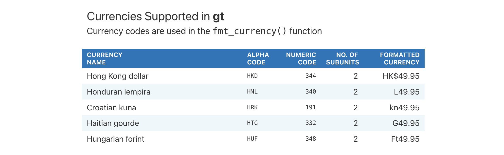
Get a table of info on all of the common currency name/symbols that can be
used with fmt_currency().
info_currencies(type = "symbol")
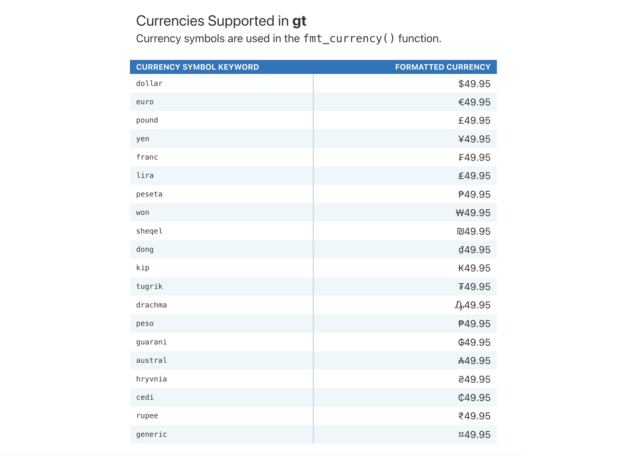
Function ID
11-3
Function Introduced
v0.2.0.5 (March 31, 2020)
See Also
Other information functions:
info_date_style(),
info_flags(),
info_google_fonts(),
info_icons(),
info_locales(),
info_paletteer(),
info_tf_style(),
info_time_style(),
info_unit_conversions()
View a table with info on date styles
Description
fmt_date() lets us format date-based values in a convenient manner using
preset styles. The table generated by info_date_style() provides a quick
reference to all styles, with associated format names and example outputs
using a fixed date (2000-02-29).
Usage
info_date_style(locale = NULL)info_date_style(locale = NULL)
Arguments
locale |
Locale identifier
An optional locale identifier that can be used for displaying formatted
date values according to the locale's rules. Examples include |
Value
An object of class gt_tbl.
Examples
Get a table of info on the different date-formatting styles (which are used
by supplying a number code to fmt_date()).
info_date_style()
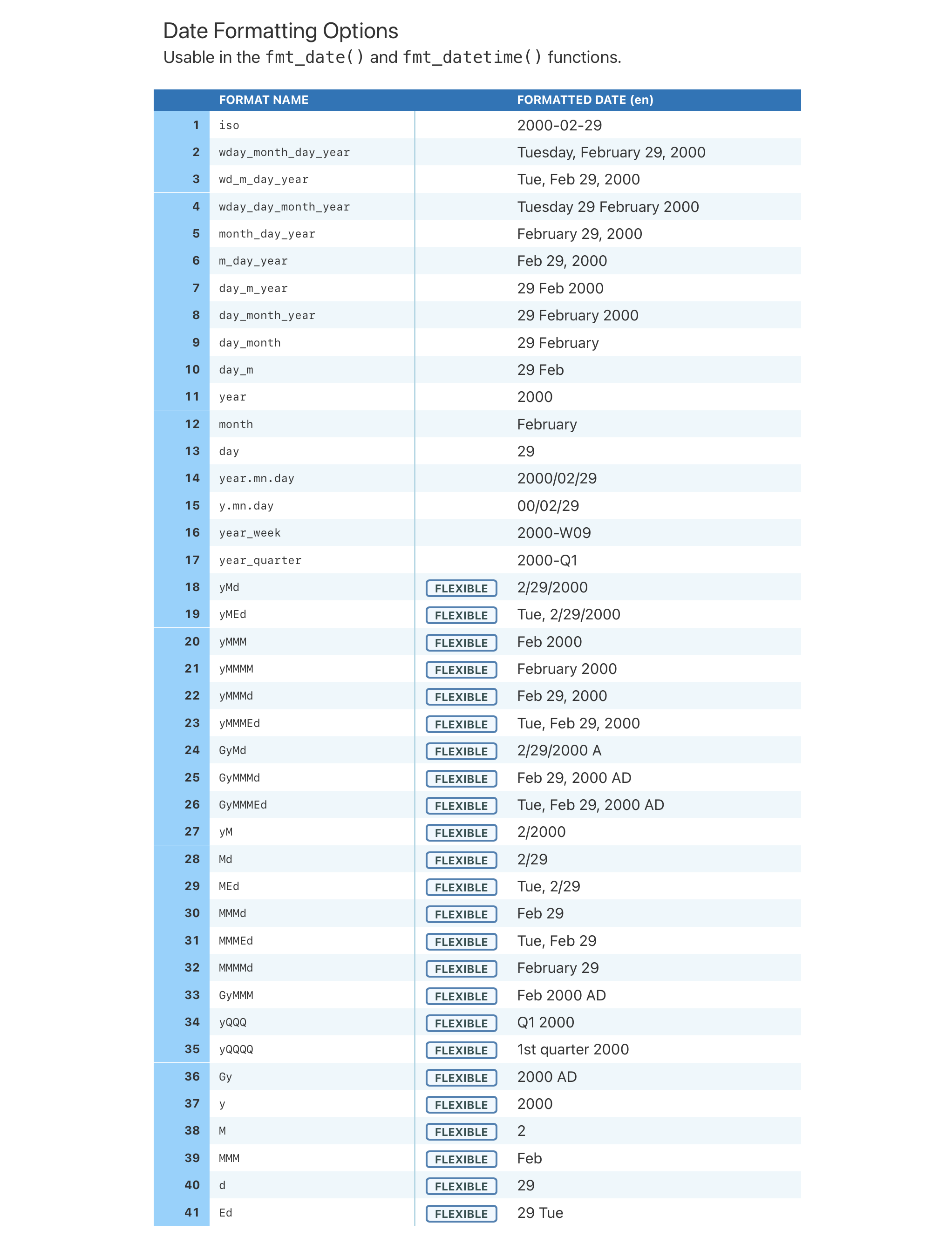
Function ID
11-1
Function Introduced
v0.2.0.5 (March 31, 2020)
See Also
Other information functions:
info_currencies(),
info_flags(),
info_google_fonts(),
info_icons(),
info_locales(),
info_paletteer(),
info_tf_style(),
info_time_style(),
info_unit_conversions()
View a table with all available flags for fmt_flag()
Description
fmt_flag() can be used to render flag icons within body cells that have
2-letter country codes. There are a lot of countries, so, calling
info_flags() can be helpful in showing all of the valid and supported
country codes along with their flag icons.
Usage
info_flags()info_flags()
Value
An object of class gt_tbl.
Examples
Get a table of info on all the available flag icons.
info_flags()
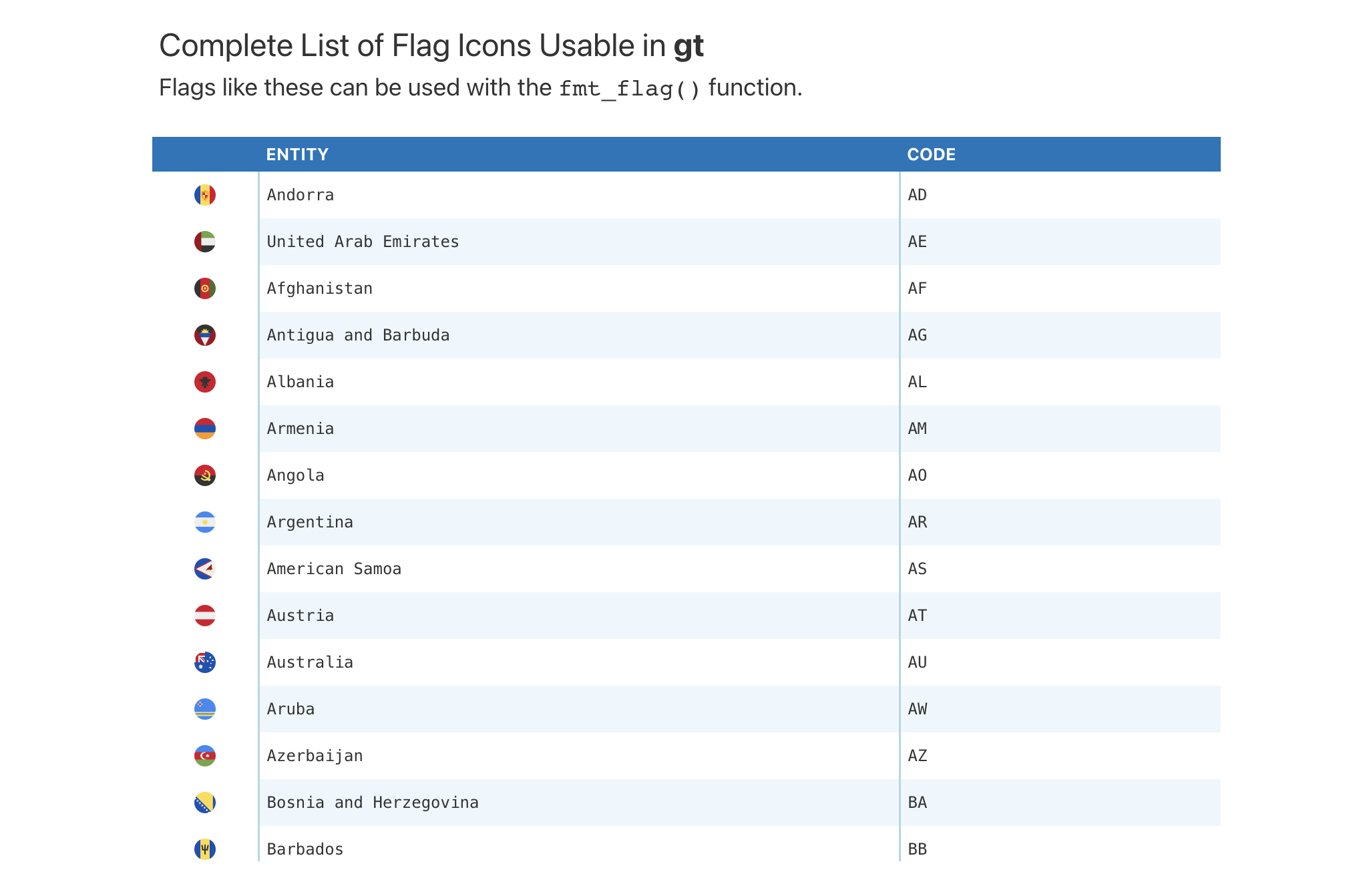
Function ID
11-8
Function Introduced
v0.10.0 (October 7, 2023)
See Also
Other information functions:
info_currencies(),
info_date_style(),
info_google_fonts(),
info_icons(),
info_locales(),
info_paletteer(),
info_tf_style(),
info_time_style(),
info_unit_conversions()
View a table on recommended Google Fonts
Description
The google_font() helper function can be used wherever a font name should
be specified. There are two instances where this helper can be used: the
name argument in opt_table_font() (for setting a table font) and in that
of cell_text() (used with tab_style()). Because there is an overwhelming
number of fonts available in the Google Fonts catalog, the
info_google_fonts() provides a table with a set of helpful font
recommendations. These fonts look great in the different parts of a gt
table. Why? For the most part they are suitable for body text, having large
counters, large x-height, reasonably low contrast, and open apertures. These
font features all make for high legibility at smaller sizes.
Usage
info_google_fonts()info_google_fonts()
Value
An object of class gt_tbl.
Examples
Get a table of info on some of the recommended Google Fonts for tables.
info_google_fonts()
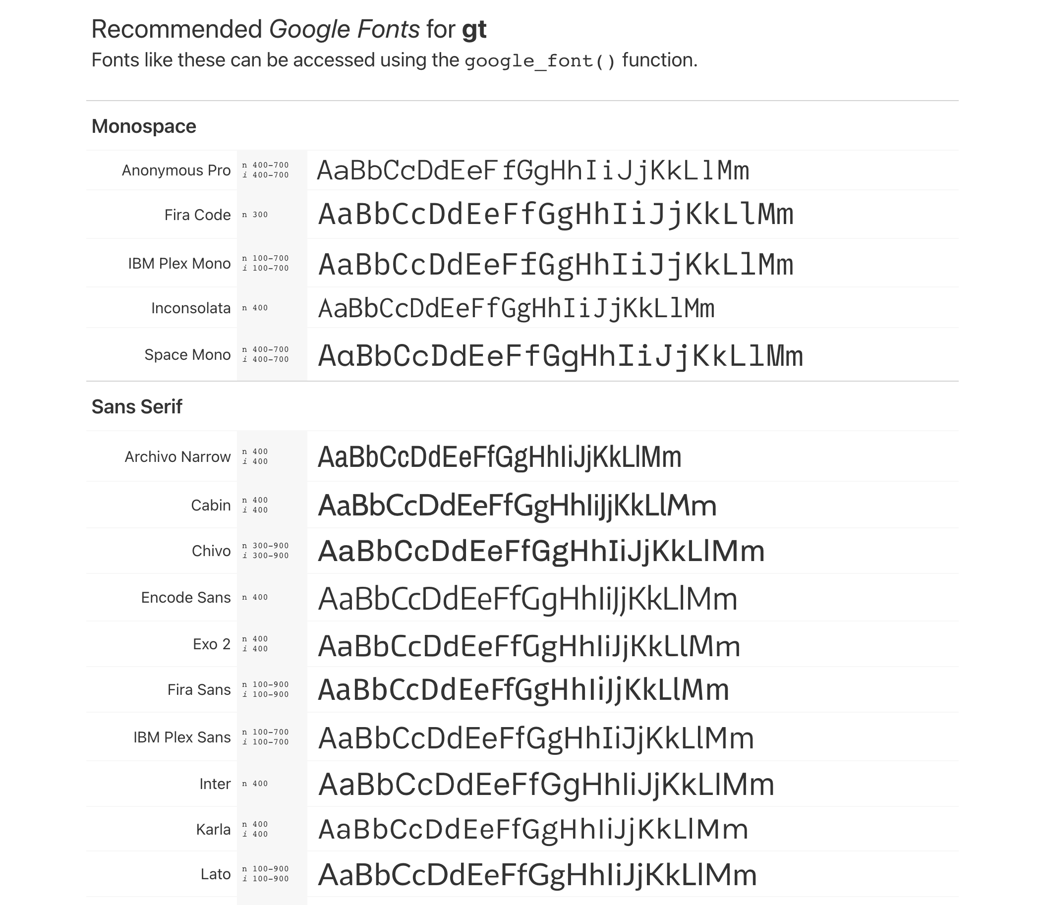
Function ID
11-6
Function Introduced
v0.2.2 (August 5, 2020)
See Also
Other information functions:
info_currencies(),
info_date_style(),
info_flags(),
info_icons(),
info_locales(),
info_paletteer(),
info_tf_style(),
info_time_style(),
info_unit_conversions()
View a table with all available Font Awesome icons for fmt_icon()
Description
fmt_icon() can be used to render Font Awesome icons within
body cells that reference the icon names. Further to this, the text
transformation functions (e.g., text_case_match()) allow for the insertion
of these icons as replacement text (so long as you use the fa() function
from the fontawesome package). Because there is a very large number of
icons available to use in Font Awesome, info_icons() can be used to
provide us with a table that lists all the icons along with their short and
full names (either can be used with fmt_icon()). It also contains
acceptable codes for fmt_country()
Usage
info_icons()info_icons()
Value
An object of class gt_tbl.
Examples
Get a table of info on all the available Font Awesome icons.
info_icons()
Function ID
11-9
Function Introduced
v0.10.0 (October 7, 2023)
See Also
Other information functions:
info_currencies(),
info_date_style(),
info_flags(),
info_google_fonts(),
info_locales(),
info_paletteer(),
info_tf_style(),
info_time_style(),
info_unit_conversions()
View a table with info on supported locales
Description
Many of the fmt_*() functions have a locale argument that makes
locale-based formatting easier. The table generated by the info_locales()
function provides a quick reference to all the available locales. The locale
identifiers are provided (base locale ID, common display name) along with the
each locale's group and decimal separator marks. A formatted numeric example
is provided (based on the value of 11027) to demonstrate the default
formatting of each locale.
Usage
info_locales(begins_with = NULL)info_locales(begins_with = NULL)
Arguments
begins_with |
Show locales beginning with a specific letter
Providing a single letter will filter locales to only those that begin
with that letter in their locale ID. The default ( |
Details
There are 574 locales, which means that a very long display
table is provided by default. To trim down the output table size, we can
provide an initial letter corresponding to the base locale ID to
begins_with. This will filter locales in the info table to just the set
that begins with the supplied letter.
Value
An object of class gt_tbl.
Examples
Get a table of info on all of the locales supported by gt.
info_locales()
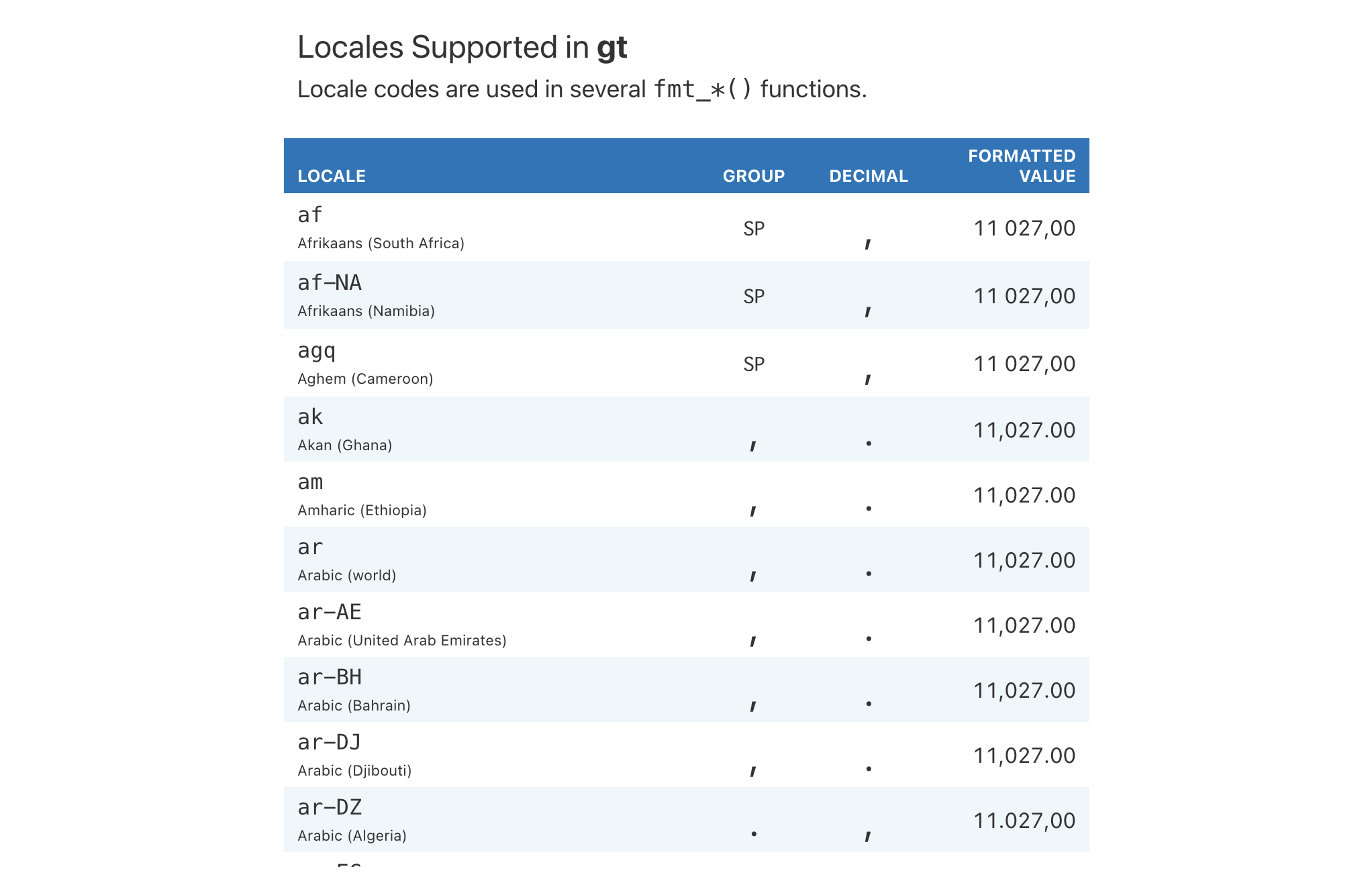
Function ID
11-4
Function Introduced
v0.2.0.5 (March 31, 2020)
See Also
Other information functions:
info_currencies(),
info_date_style(),
info_flags(),
info_google_fonts(),
info_icons(),
info_paletteer(),
info_tf_style(),
info_time_style(),
info_unit_conversions()
View a table with info on color palettes
Description
While data_color() allows us to flexibly color data cells in our gt
table, the harder part of this process is discovering and choosing color
palettes that are suitable for the table output. We can make this process
much easier in two ways: (1) by using the paletteer package, which makes
a wide range of palettes from various R packages readily available, and (2)
calling info_paletteer() to give us an information table that serves as a
quick reference for all of the discrete color palettes available in
paletteer.
Usage
info_paletteer(color_pkgs = NULL)info_paletteer(color_pkgs = NULL)
Arguments
color_pkgs |
Filter to specific color packages
A vector of color packages that determines which sets of palettes should be
displayed in the information table. If this is |
Details
The palettes displayed are organized by package and by palette name. These
values are required when obtaining a palette (as a vector of hexadecimal
colors), from paletteer::paletteer_d(). Once we are familiar with the names
of the color palette packages (e.g., RColorBrewer, ggthemes,
wesanderson), we can narrow down the content of this information table by
supplying a vector of such package names to color_pkgs.
Colors from the following color packages (all supported by paletteer)
are shown by default with info_paletteer():
-
awtools, 5 palettes
-
dichromat, 17 palettes
-
dutchmasters, 6 palettes
-
ggpomological, 2 palettes
-
ggsci, 42 palettes
-
ggthemes, 31 palettes
-
ghibli, 27 palettes
-
grDevices, 1 palette
-
jcolors, 13 palettes
-
LaCroixColoR, 21 palettes
-
NineteenEightyR, 12 palettes
-
nord, 16 palettes
-
ochRe, 16 palettes
-
palettetown, 389 palettes
-
pals, 8 palettes
-
Polychrome, 7 palettes
-
quickpalette, 17 palettes
-
rcartocolor, 34 palettes
-
RColorBrewer, 35 palettes
-
Redmonder, 41 palettes
-
wesanderson, 19 palettes
-
yarrr, 21 palettes
Value
An object of class gt_tbl.
Examples
Get a table of info on just the "ggthemes" color palette (easily accessible
from the paletteer package).
info_paletteer(color_pkgs = "ggthemes")
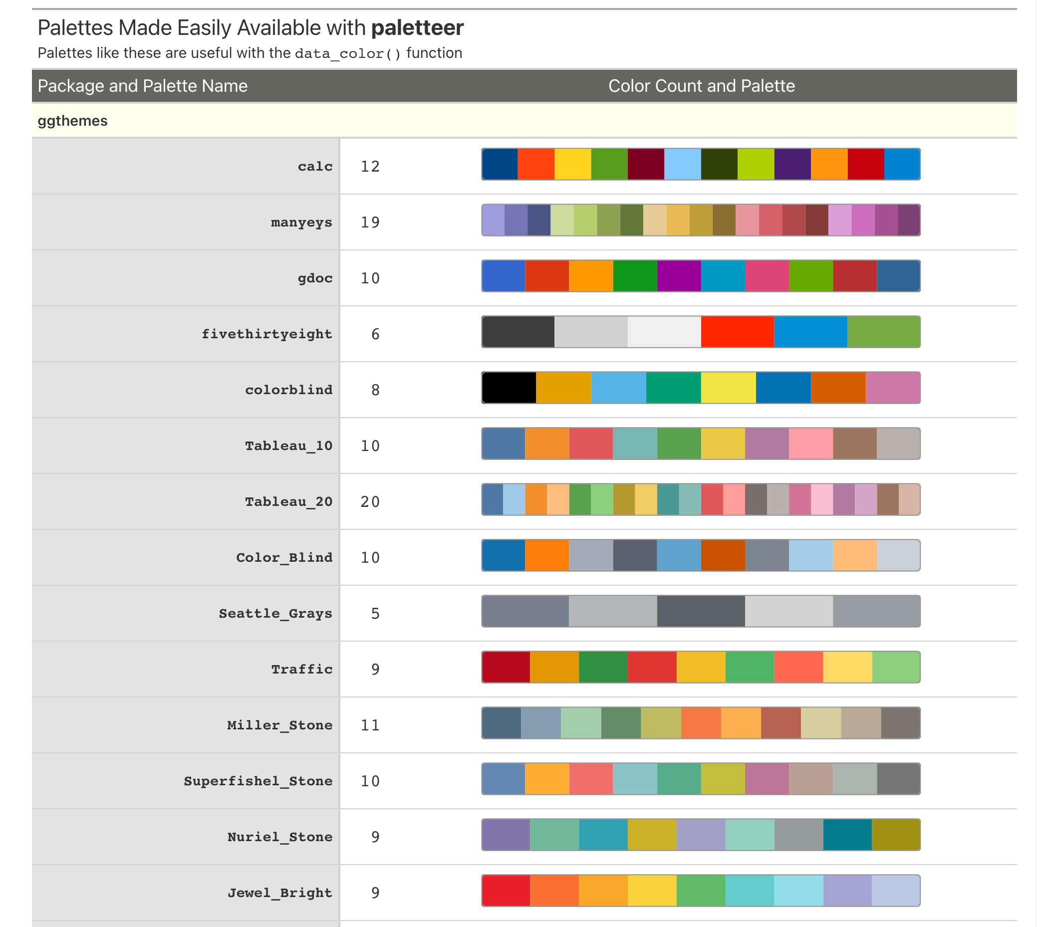
Function ID
11-5
Function Introduced
v0.2.0.5 (March 31, 2020)
See Also
Other information functions:
info_currencies(),
info_date_style(),
info_flags(),
info_google_fonts(),
info_icons(),
info_locales(),
info_tf_style(),
info_time_style(),
info_unit_conversions()
View a table with info on TRUE/FALSE formatting styles
Description
fmt_tf() lets us format logical values in a convenient manner using preset
styles. The table generated by info_tf_style() provides a quick reference
to all styles, with associated format names and example output values.
Usage
info_tf_style(locale = NULL)info_tf_style(locale = NULL)
Arguments
locale |
Locale identifier
An optional locale identifier that can be used for displaying formatted
TRUE/FALSE values according to the locale's rules. Examples include |
Value
An object of class gt_tbl.
Examples
Get a table of info on the different TRUE/FALSE-formatting styles (which
are used by supplying a number code or format name to fmt_tf()).
info_tf_style()
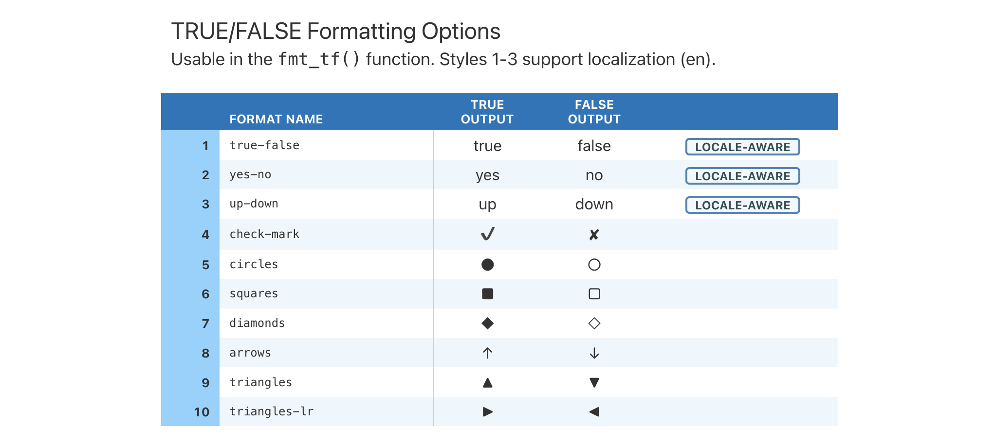
Function ID
11-7
Function Introduced
v1.3.0 (January 22, 2026)
See Also
Other information functions:
info_currencies(),
info_date_style(),
info_flags(),
info_google_fonts(),
info_icons(),
info_locales(),
info_paletteer(),
info_time_style(),
info_unit_conversions()
View a table with info on time styles
Description
fmt_time() lets us format time-based values in a convenient manner using
preset styles. The table generated by info_time_style() provides a quick
reference to all styles, with associated format names and example outputs
using a fixed time (14:35).
Usage
info_time_style(locale = NULL)info_time_style(locale = NULL)
Arguments
locale |
Locale identifier
An optional locale identifier that can be used for displaying formatted
time values according to the locale's rules. Examples include |
Value
An object of class gt_tbl.
Examples
Get a table of info on the different time-formatting styles (which are used
by supplying a number code to fmt_time()).
info_time_style()
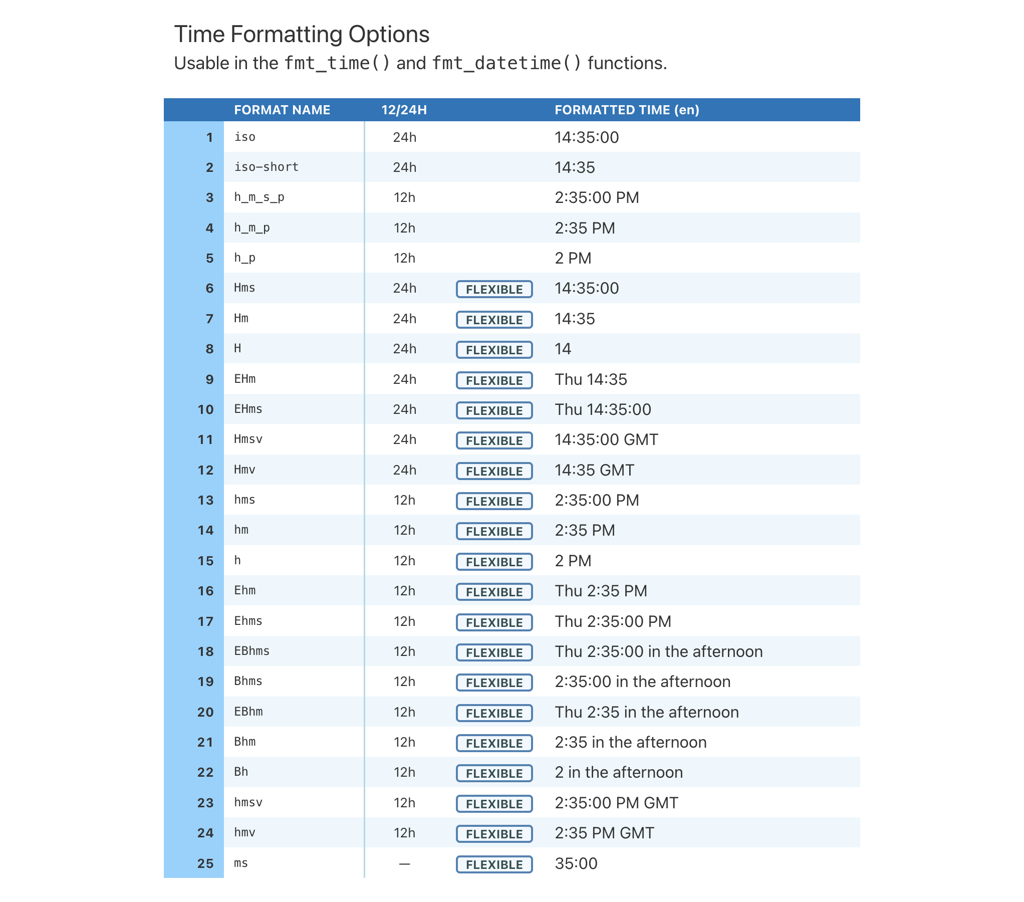
Function ID
11-2
Function Introduced
v0.2.0.5 (March 31, 2020)
See Also
Other information functions:
info_currencies(),
info_date_style(),
info_flags(),
info_google_fonts(),
info_icons(),
info_locales(),
info_paletteer(),
info_tf_style(),
info_unit_conversions()
View a table with all units that can be converted by unit_conversion()
Description
unit_conversion() can be used to yield conversion factors across compatible
pairs of units. This is useful for expressing values in different units and
the conversion can be performed via the scale_by argument available in
several formatting functions. When calling unit_conversion(), one must
supply two string-based keywords to specify the value's current units and the
desired units. All of these keywords are provided in the table shown by
calling info_unit_conversions().
Usage
info_unit_conversions()info_unit_conversions()
Value
An object of class gt_tbl.
Examples
Get a table of info on all the available keywords for unit conversions.
info_unit_conversions()

Function ID
11-10
Function Introduced
v0.11.0 (July 9, 2024)
See Also
Other information functions:
info_currencies(),
info_date_style(),
info_flags(),
info_google_fonts(),
info_icons(),
info_locales(),
info_paletteer(),
info_tf_style(),
info_time_style()
Interpret input text as LaTeX-formatted text
Description
For certain pieces of text (like in column labels or table headings) we may
want to express them as raw LaTeX. In fact, with LaTeX, so much more can be done for formatting.
The latex() function will guard the input LaTeX from being escaped.
Usage
latex(text)latex(text)
Arguments
text |
LaTeX text
The text that is understood to be LaTeX text, which is to be preserved in the LaTeX output context. |
Value
A character object of class latex. It's tagged as an latex fragment
that is not to be sanitized.
Examples
Use the exibble dataset to create a gt table. When adding a title
through tab_header(), we'll use the latex() helper to signify to gt
that we're using LaTeX formatting.
exibble |>
dplyr::select(currency, char) |>
gt() |>
tab_header(title = latex("\\emph{LaTeX}"))
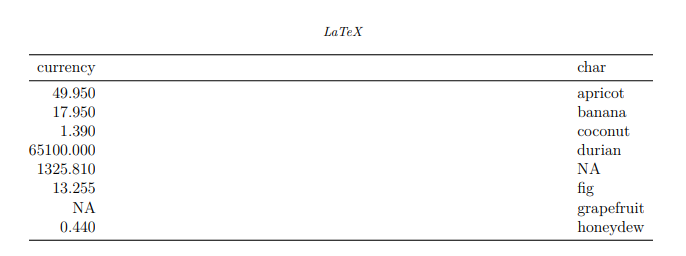
Function ID
8-2
Function Introduced
v1.0.1 (May 10, 2025)
See Also
Other helper functions:
adjust_luminance(),
cell_borders(),
cell_fill(),
cell_text(),
currency(),
default_fonts(),
escape_latex(),
from_column(),
google_font(),
gt_latex_dependencies(),
html(),
md(),
nanoplot_options(),
pct(),
px(),
random_id(),
row_group(),
stub(),
system_fonts(),
unit_conversion()
Helper function for adding a local image
Description
We can flexibly add a local image (i.e., an image residing on disk) inside of
a table with local_image() function. The function provides a convenient way
to generate an HTML fragment using an on-disk PNG or SVG. Because this
function is currently HTML-based, it is only useful for HTML table output. To
use this function inside of data cells, it is recommended to use
text_transform() first. With that function, we can specify which data cells
to target and then include a local_image() call within the required
user-defined function (for the fn argument). If we want to include an image
in other places (e.g., in the header, within footnote text, etc.) we need to
use local_image() within the html() helper function.
By itself, the function creates an HTML image tag with an image URI embedded
within. We can easily experiment with a local PNG or SVG image that's
available in the gt package using the test_image() function. Using
that, the call local_image(file = test_image(type = "png")) evaluates to:
<img src=<data URI> style=\"height:30px;\">
where a height of 30px is a default height chosen to work well within the
heights of most table rows.
Usage
local_image(filename, height = 30)local_image(filename, height = 30)
Arguments
filename |
Path to image file
A local path to an image file on disk. |
height |
Height of image
The absolute height of the image in the table cell (in |
Value
A character object with an HTML fragment that can be placed inside of a cell.
Examples
Create a tibble that contains heights of an image in pixels (one column as a
string, the other as numerical values), then, create a gt table. Use
text_transform() to insert a local test image (PNG) image with the various
sizes.
dplyr::tibble(
pixels = px(seq(10, 35, 5)),
image = seq(10, 35, 5)
) |>
gt() |>
text_transform(
locations = cells_body(columns = image),
fn = function(x) {
local_image(
filename = test_image(type = "png"),
height = as.numeric(x)
)
}
)

Function ID
9-2
Function Introduced
v0.2.0.5 (March 31, 2020)
See Also
Other image addition functions:
ggplot_image(),
test_image(),
web_image()
Localize formatting and symbols
Description
Localize formatting and symbols
Specify locale
gt(), some cols_*() and fmt_*() functions have a locale argument.
You can pass locale as a 2 letters string or 4. (e.g. "fr" for French,
"pt-BR" for Brazilian Portuguese). gt also resolves different spellings
internally as much as possible. For example "en_GB" will work out of the
box.
Range of action of locale
One of the advantage of using gt its consistency in using symbols and currencies in multiple languages
There are two ways to localize your results with gt.
-
Passing it globally
gt(locale = "<locale>")
Will localize everything possible in the gt() pipeline.
-
In individual
fmt_()functions -
Localize buttons in
opt_interactive()
Will only affect the output of one specific function (or override global setting).
locale has very low precedence usually. As soon as you override some parameters,
sep_mark, dec_mark, incl_space, they will be override locale.
See Also
Examples
# The Spanish locale uses `.` as thousands sep (English uses `,`) and uses # a `,` as the decimal mark # Using the locale in `gt()` will format automatically all output in # subsequent `fmt_*()` calls. exibble |> gt(locale = "es-AR") |> fmt_number() # Only format currency as Mexican peso exibble |> gt(locale = "fr") |> fmt_currency(currency, locale = "es-MX") # will use the provided `sep_mark` exibble |> gt(locale = "fr") |> fmt_currency(currency, sep_mark = "", locale = "es-MX") # Use your imagination, and mix and match.# The Spanish locale uses `.` as thousands sep (English uses `,`) and uses # a `,` as the decimal mark # Using the locale in `gt()` will format automatically all output in # subsequent `fmt_*()` calls. exibble |> gt(locale = "es-AR") |> fmt_number() # Only format currency as Mexican peso exibble |> gt(locale = "fr") |> fmt_currency(currency, locale = "es-MX") # will use the provided `sep_mark` exibble |> gt(locale = "fr") |> fmt_currency(currency, sep_mark = "", locale = "es-MX") # Use your imagination, and mix and match.
Interpret input text as Markdown-formatted text
Description
Markdown text can be used in certain places in a gt table, and this is
wherever new text is defined (e.g., footnotes, source notes, the table title,
etc.). Using Markdown is advantageous for styling text since it will be
rendered correctly to the output format of the gt table. There is
also the html() helper that allows you use HTML exclusively (for tables
expressly meant for HTML output) but md() allows for both; you get to use
Markdown plus any HTML fragments at the same time.
Usage
md(text)md(text)
Arguments
text |
Markdown text
The text that is understood to contain Markdown formatting. |
Value
A character object of class from_markdown. It's tagged as being
Markdown text and it will undergo conversion to the desired output context.
Examples
Use the exibble dataset to create a gt table. When adding a title
through tab_header(), we'll use the md() helper to signify to gt that
we're using Markdown formatting.
exibble |>
dplyr::select(currency, char) |>
gt() |>
tab_header(title = md("Using *Markdown*"))

Function ID
8-1
Function Introduced
v0.2.0.5 (March 31, 2020)
See Also
Other helper functions:
adjust_luminance(),
cell_borders(),
cell_fill(),
cell_text(),
currency(),
default_fonts(),
escape_latex(),
from_column(),
google_font(),
gt_latex_dependencies(),
html(),
latex(),
nanoplot_options(),
pct(),
px(),
random_id(),
row_group(),
stub(),
system_fonts(),
unit_conversion()
The stations of the Paris Metro
Description
A dataset with information on all 321 Paris Metro stations as of August 2025. Each record represents a station, describing which Metro lines are serviced by the station, which other connections are available, and annual passenger volumes. Basic location information is provided for each station in terms of where they reside on a municipal level, and, through latitude/longitude coordinate values.
The system has 16 lines (numbered from 1 to 14, with two additional lines: 3bis and 7bis) and covers over 200 kilometers of track. The Metro runs on standard gauge tracks (1,435 mm) and operates using a variety of rolling stock, including rubber-tired trains and steel-wheeled trains (which are far more common).
The Metro is operated by the RATP, which also operates other transit systems in the region, including buses, trams, and the RER. The RER is an important component of the region's transit infrastructure, and several RER stations have connectivity with the Metro. This integration allows passengers to transfer between those two systems seamlessly. The Metro also has connections to the Transilien rail network, tramway stations, several major train stations (e.g., Gare du Nord, Gare de l'Est, etc.), and many bus lines.
Usage
metrometro
Format
A tibble with 321 rows and 11 variables:
- name
-
The name of the station.
- caption
-
In some cases, a station will have a caption that might describe a nearby place of interest. This is
NAif there isn't a caption for the station name. - lines
-
All Metro lines associated with the station. This is a
character-based, comma-separated series of line names. - connect_rer
-
Station connections with the RER. The RER system has five lines (A, B, C, D, and E) with 257 stations and several interchanges with the Metro.
- connect_tram
-
Connections with tramway lines. This system has twelve lines in operation (T1, T2, T3a, T3b, T4, T5, T6, T7, T8, T9, T11, and T13) with 235 stations.
- connect_transilien
-
Connections with Transilien lines. This system has eight lines in operation (H, J, K, L, N, P, R, and U).
- connect_other
-
Other connections with transportation infrastructure such as regional, intercity, night, and high-speed trains (typically at railway stations).
- latitude, longitude
-
The location of the station, given as latitude and longitude values in decimal degrees.
- location
-
The arrondissement of Paris or municipality in which the station resides. For some stations located at borders, the grouping of locations will be presented as a comma-separated series
- passengers
-
The total number of Metro station entries during 2021. Some of the newest stations in the Metro system do not have this data, thus they show
NAvalues.
Dataset ID and Badge
DATA-10

Dataset Introduced
v0.9.0 (Mar 31, 2023)
See Also
Other datasets:
constants,
countrypops,
exibble,
films,
gibraltar,
gtcars,
illness,
nuclides,
peeps,
photolysis,
pizzaplace,
reactions,
rx_addv,
rx_adsl,
sp500,
sza,
towny
Examples
dplyr::glimpse(metro)dplyr::glimpse(metro)
Supply nanoplot options to cols_nanoplot()
Description
When using cols_nanoplot(), the defaults for the generated nanoplots
can be modified with nanoplot_options() within the options argument.
Usage
nanoplot_options( data_point_radius = NULL, data_point_stroke_color = NULL, data_point_stroke_width = NULL, data_point_fill_color = NULL, data_line_type = NULL, data_line_stroke_color = NULL, data_line_stroke_width = NULL, data_area_fill_color = NULL, data_bar_stroke_color = NULL, data_bar_stroke_width = NULL, data_bar_fill_color = NULL, data_bar_negative_stroke_color = NULL, data_bar_negative_stroke_width = NULL, data_bar_negative_fill_color = NULL, reference_line_color = NULL, reference_area_fill_color = NULL, vertical_guide_stroke_color = NULL, vertical_guide_stroke_width = NULL, show_data_points = NULL, show_data_line = NULL, show_data_area = NULL, show_reference_line = NULL, show_reference_area = NULL, show_vertical_guides = NULL, show_y_axis_guide = NULL, interactive_data_values = NULL, y_val_fmt_fn = NULL, y_axis_fmt_fn = NULL, y_ref_line_fmt_fn = NULL, currency = NULL )nanoplot_options( data_point_radius = NULL, data_point_stroke_color = NULL, data_point_stroke_width = NULL, data_point_fill_color = NULL, data_line_type = NULL, data_line_stroke_color = NULL, data_line_stroke_width = NULL, data_area_fill_color = NULL, data_bar_stroke_color = NULL, data_bar_stroke_width = NULL, data_bar_fill_color = NULL, data_bar_negative_stroke_color = NULL, data_bar_negative_stroke_width = NULL, data_bar_negative_fill_color = NULL, reference_line_color = NULL, reference_area_fill_color = NULL, vertical_guide_stroke_color = NULL, vertical_guide_stroke_width = NULL, show_data_points = NULL, show_data_line = NULL, show_data_area = NULL, show_reference_line = NULL, show_reference_area = NULL, show_vertical_guides = NULL, show_y_axis_guide = NULL, interactive_data_values = NULL, y_val_fmt_fn = NULL, y_axis_fmt_fn = NULL, y_ref_line_fmt_fn = NULL, currency = NULL )
Arguments
data_point_radius |
Radius of data points
The |
data_point_stroke_color |
Color of data points
The default stroke color of the data points is |
data_point_stroke_width |
Width of surrounding line on data points
The width of the outside stroke for the data points can be modified with
the |
data_point_fill_color |
Fill color for data points
By default, all data points have a fill color of |
data_line_type |
Type of data line: curved or straight
This can accept either |
data_line_stroke_color |
Color of the data line
The color of the data line can be modified from its default |
data_line_stroke_width |
Width of the data line
The width of the connecting data line can be modified with the
|
data_area_fill_color |
Fill color for the data-point-bounded area
The fill color for the area that bounds the data points in line plot. The
default is |
data_bar_stroke_color |
Color of a data bar's outside line
The color of the stroke used for the data bars can be modified from its
default |
data_bar_stroke_width |
Width of a data bar's outside line
The width of the stroke used for the data bars can be modified with the
|
data_bar_fill_color |
Fill color for data bars
By default, all data bars have a fill color of |
data_bar_negative_stroke_color |
Stroke color for negative values
The color of the stroke used for the data bars that have negative values.
The default color is |
data_bar_negative_stroke_width |
Stroke width for negative values
The width of the stroke used for negative value data bars. This has the
same default as |
data_bar_negative_fill_color |
Fill color for negative values
By default, all negative data bars have a fill color of |
reference_line_color |
Color for the reference line
The reference line will have a color of |
reference_area_fill_color |
Fill color for the reference area
If a reference area has been defined and is visible it has by default
a fill color of |
vertical_guide_stroke_color |
Color of vertical guides
Vertical guides appear when hovering in the vicinity of data points. Their
default color is |
vertical_guide_stroke_width |
Line widths for vertical guides
The vertical guide's stroke width, by default, is relatively large at |
show_data_points |
Should the data points be shown?
By default, all data points in a nanoplot are shown but this layer can be
hidden by setting |
show_data_line |
Should a data line be shown?
The data line connects data points together and it is shown by default.
This data line layer can be hidden by setting |
show_data_area |
Should a data-point-bounded area be shown?
The data area layer is adjacent to the data points and the data line. It is
shown by default but can be hidden with |
show_reference_line |
Should a reference line be shown?
The layer with a horizontal reference line appears underneath that of the
data points and the data line. Like vertical guides, hovering over a
reference will show its value. The reference line (if available) is shown
by default but can be hidden by setting |
show_reference_area |
Should a reference area be shown?
The reference area appears at the very bottom of the layer stack, if it is
available (i.e., defined in |
show_vertical_guides |
Should there be vertical guides?
Vertical guides appear when hovering over data points. This hidden layer is
active by default but can be deactivated by using
|
show_y_axis_guide |
Should there be a y-axis guide?
The y-axis guide will appear when hovering over the far left side of a
nanoplot. This hidden layer is active by default but can be deactivated by
using |
interactive_data_values |
Should data values be interactively shown?
By default, numeric data values will be shown only when the user interacts
with certain regions of a nanoplot. This is because the values may be
numerous (i.e., clutter the display when all are visible) and it can be
argued that the values themselves are secondary to the presentation.
However, for some types of plots (like horizontal bar plots), a persistent
display of values alongside the plot marks may be desirable. By setting
|
y_val_fmt_fn, y_axis_fmt_fn, y_ref_line_fmt_fn
|
Custom formatting for y values
If providing a function to |
currency |
Define values as currencies of a specific type
If the values are to be displayed as currency values, supply either: (1) a
3-letter currency code (e.g., |
Value
A list object of class nanoplot_options.
Function ID
8-8
Function Introduced
v0.10.0 (October 7, 2023)
See Also
Other helper functions:
adjust_luminance(),
cell_borders(),
cell_fill(),
cell_text(),
currency(),
default_fonts(),
escape_latex(),
from_column(),
google_font(),
gt_latex_dependencies(),
html(),
latex(),
md(),
pct(),
px(),
random_id(),
row_group(),
stub(),
system_fonts(),
unit_conversion()
Nuclide data
Description
The nuclides dataset contains information on all known nuclides, providing
data on nuclear structure and decay modes across 118 elements. There is data
here on natural abundances, atomic mass, spin, half-life, and more. The
typical users for such a dataset include researchers in fields such as
nuclear physics, radiochemistry, and nuclear medicine.
Usage
nuclidesnuclides
Format
A tibble with 3,383 rows and 29 variables:
- nuclide
-
The symbol for the nuclide.
- z, n
-
The number of protons and neutrons.
- element
-
The element symbol.
- radius, radius_uncert
-
The charge radius and its associated uncertainty. In units of fm.
- abundance, abundance_uncert
-
The abundance of the stable isotope as a mole fraction (in relation to other stable isotopes of the same element). Values are provided for the nuclide only if
is_stableisTRUE. - is_stable
-
Is the nuclide a stable isotope?
- half_life, half_life_uncert
-
The nuclide's half life represented as seconds.
- isospin
-
The isospin, or the quantum number related to the up and down quark content of the particle.
- decay_1, decay_2, decay_3
-
The 1st, 2nd, and 3rd decay modes.
- decay_1_pct, decay_1_pct_uncert, decay_2_pct, decay_2_pct_uncert, decay_3_pct, decay_3_pct_uncert
-
The branching proportions for the 1st, 2nd, and 3rd decays (along with uncertainty values).
- magnetic_dipole, magnetic_dipole_uncert
-
The magnetic dipole and its associated uncertainty. Expressed in units of micro N, or nuclear magneton values.
- electric_quadrupole, electric_quadrupole_uncert
-
The electric quadrupole and its associated uncertainty. In units of barn (b).
- atomic_mass, atomic_mass_uncert
-
The atomic mass and its associated uncertainty. In units of micro AMU.
- mass_excess, mass_excess_uncert
-
The mass excess and its associated uncertainty. In units of keV.
Dataset ID and Badge
DATA-16

Dataset Introduced
v0.11.0 (July 9, 2024)
See Also
Other datasets:
constants,
countrypops,
exibble,
films,
gibraltar,
gtcars,
illness,
metro,
peeps,
photolysis,
pizzaplace,
reactions,
rx_addv,
rx_adsl,
sp500,
sza,
towny
Examples
dplyr::glimpse(nuclides)dplyr::glimpse(nuclides)
Option to align the table header
Description
By default, a table header added to a gt table has center alignment
for both the title and the subtitle elements. This function allows us to
easily set the horizontal alignment of the title and subtitle to the left
or right by using the "align" argument. This function serves as a
convenient shortcut for <gt_tbl> |> tab_options(heading.align = <align>).
Usage
opt_align_table_header(data, align = c("left", "center", "right"))opt_align_table_header(data, align = c("left", "center", "right"))
Arguments
data |
The gt table data object
This is the gt table object that is commonly created through use of the
|
align |
Header alignment
The alignment of the title and subtitle elements in the table header.
Options are |
Value
An object of class gt_tbl.
Examples
Use the exibble dataset to create a gt table with a number of table
parts added (using functions like summary_rows(), grand_summary_rows(),
and more). Following that, we'll align the header contents (consisting of the
title and the subtitle) to the left with the opt_align_table_header()
function.
exibble |>
gt(rowname_col = "row", groupname_col = "group") |>
summary_rows(
groups = "grp_a",
columns = c(num, currency),
fns = c("min", "max")
) |>
grand_summary_rows(
columns = currency,
fns = total ~ sum(., na.rm = TRUE)
) |>
tab_source_note(source_note = "This is a source note.") |>
tab_footnote(
footnote = "This is a footnote.",
locations = cells_body(columns = 1, rows = 1)
) |>
tab_header(
title = "The title of the table",
subtitle = "The table's subtitle"
) |>
opt_align_table_header(align = "left")

Function ID
10-7
Function Introduced
v0.2.0.5 (March 31, 2020)
See Also
Other table option functions:
opt_all_caps(),
opt_css(),
opt_footnote_marks(),
opt_footnote_order(),
opt_footnote_spec(),
opt_horizontal_padding(),
opt_interactive(),
opt_row_striping(),
opt_stylize(),
opt_table_font(),
opt_table_lines(),
opt_table_outline(),
opt_vertical_padding()
Option to use all caps in select table locations
Description
Sometimes an all-capitalized look is suitable for a table. With the
opt_all_caps() function, we can transform characters in the column labels,
the stub, and in all row groups in this way (and there's control over which
of these locations are transformed).
This function serves as a convenient shortcut for <gt_tbl> |> tab_options(<location>.text_transform = "uppercase", <location>.font.size = pct(80), <location>.font.weight = "bolder") (for all locations selected).
Usage
opt_all_caps( data, all_caps = TRUE, locations = c("column_labels", "stub", "row_group") )opt_all_caps( data, all_caps = TRUE, locations = c("column_labels", "stub", "row_group") )
Arguments
data |
The gt table data object
This is the gt table object that is commonly created through use of the
|
all_caps |
Use all-caps transformation
A logical value to indicate whether the text transformation to all caps
should be performed ( |
locations |
Locations to target
Which locations should undergo this text transformation? By default it
includes all of the |
Value
An object of class gt_tbl.
Examples
Use the exibble dataset to create a gt table with a number of table
parts added (using functions like summary_rows(), grand_summary_rows(),
and more). Following that, we'll ensure that all text in the column labels,
the stub, and in all row groups is transformed to all caps using
opt_all_caps().
exibble |>
gt(rowname_col = "row", groupname_col = "group") |>
summary_rows(
groups = "grp_a",
columns = c(num, currency),
fns = c("min", "max")
) |>
grand_summary_rows(
columns = currency,
fns = total ~ sum(., na.rm = TRUE)
) |>
tab_source_note(source_note = "This is a source note.") |>
tab_footnote(
footnote = "This is a footnote.",
locations = cells_body(columns = 1, rows = 1)
) |>
tab_header(
title = "The title of the table",
subtitle = "The table's subtitle"
) |>
opt_all_caps()
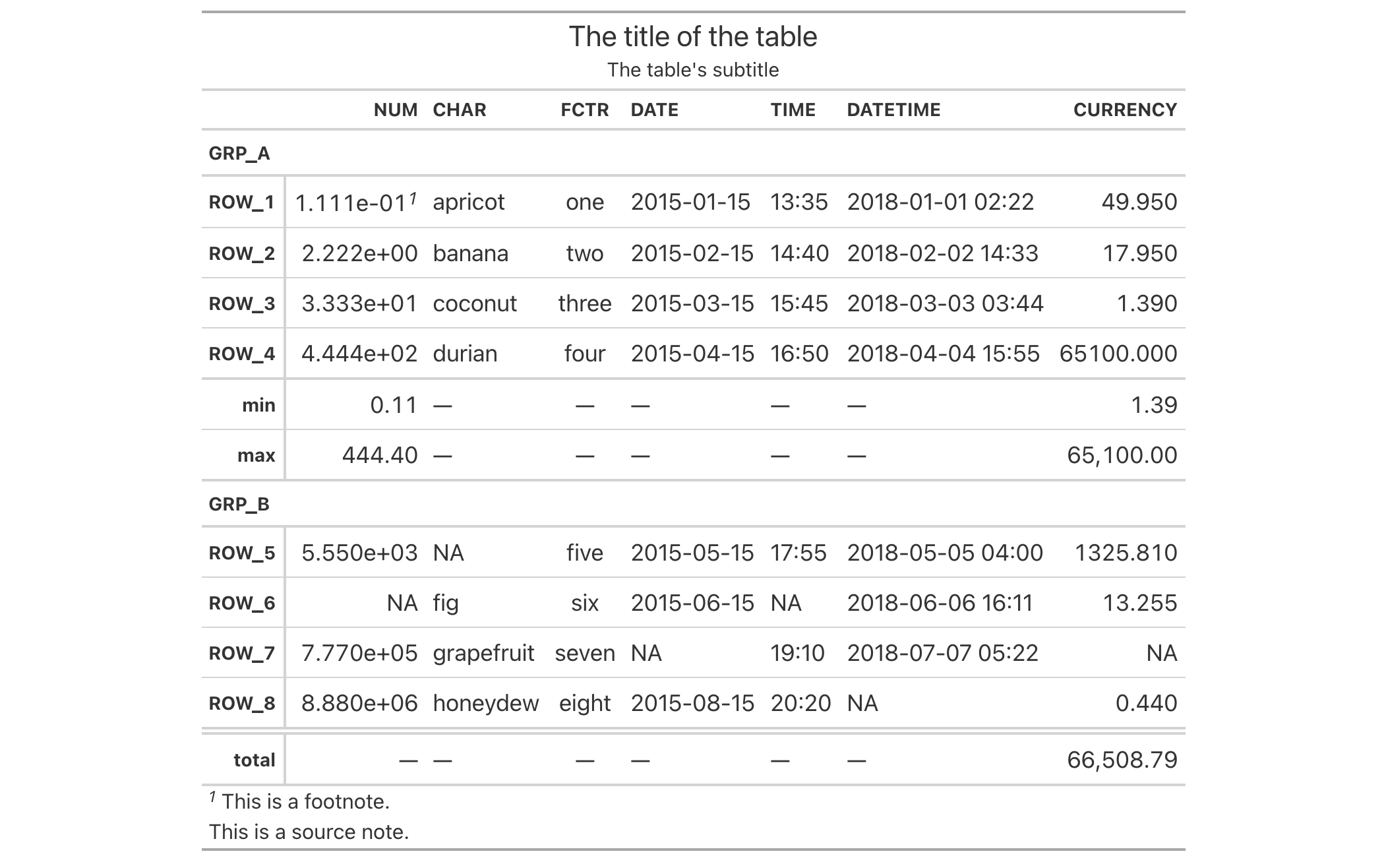
Function ID
10-10
Function Introduced
v0.2.0.5 (March 31, 2020)
See Also
Other table option functions:
opt_align_table_header(),
opt_css(),
opt_footnote_marks(),
opt_footnote_order(),
opt_footnote_spec(),
opt_horizontal_padding(),
opt_interactive(),
opt_row_striping(),
opt_stylize(),
opt_table_font(),
opt_table_lines(),
opt_table_outline(),
opt_vertical_padding()
Option to add custom CSS for the table
Description
opt_css() makes it possible to add CSS to a gt table. This CSS will be
added after the compiled CSS that gt generates automatically when the
object is transformed to an HTML output table. You can supply css as a
vector of lines or as a single string.
Usage
opt_css(data, css, add = TRUE, allow_duplicates = FALSE)opt_css(data, css, add = TRUE, allow_duplicates = FALSE)
Arguments
data |
The gt table data object
This is the gt table object that is commonly created through use of the
|
css |
CSS declarations
The CSS to include as part of the rendered table's |
add |
Add to existing CSS
If |
allow_duplicates |
Allow for CSS duplication
When this is |
Value
An object of class gt_tbl.
Examples
Let's use the exibble dataset to create a simple, two-column gt table
(keeping only the num and currency columns). Through use of the
opt_css() function, we can insert CSS rulesets as as string. We need to
ensure that the table ID is set explicitly (we've done so here with the
ID value of "one", setting it in the gt() function).
exibble |>
dplyr::select(num, currency) |>
gt(id = "one") |>
fmt_currency(
columns = currency,
currency = "HKD"
) |>
fmt_scientific(columns = num) |>
opt_css(
css = "
#one .gt_table {
background-color: skyblue;
}
#one .gt_row {
padding: 20px 30px;
}
#one .gt_col_heading {
text-align: center !important;
}
"
)
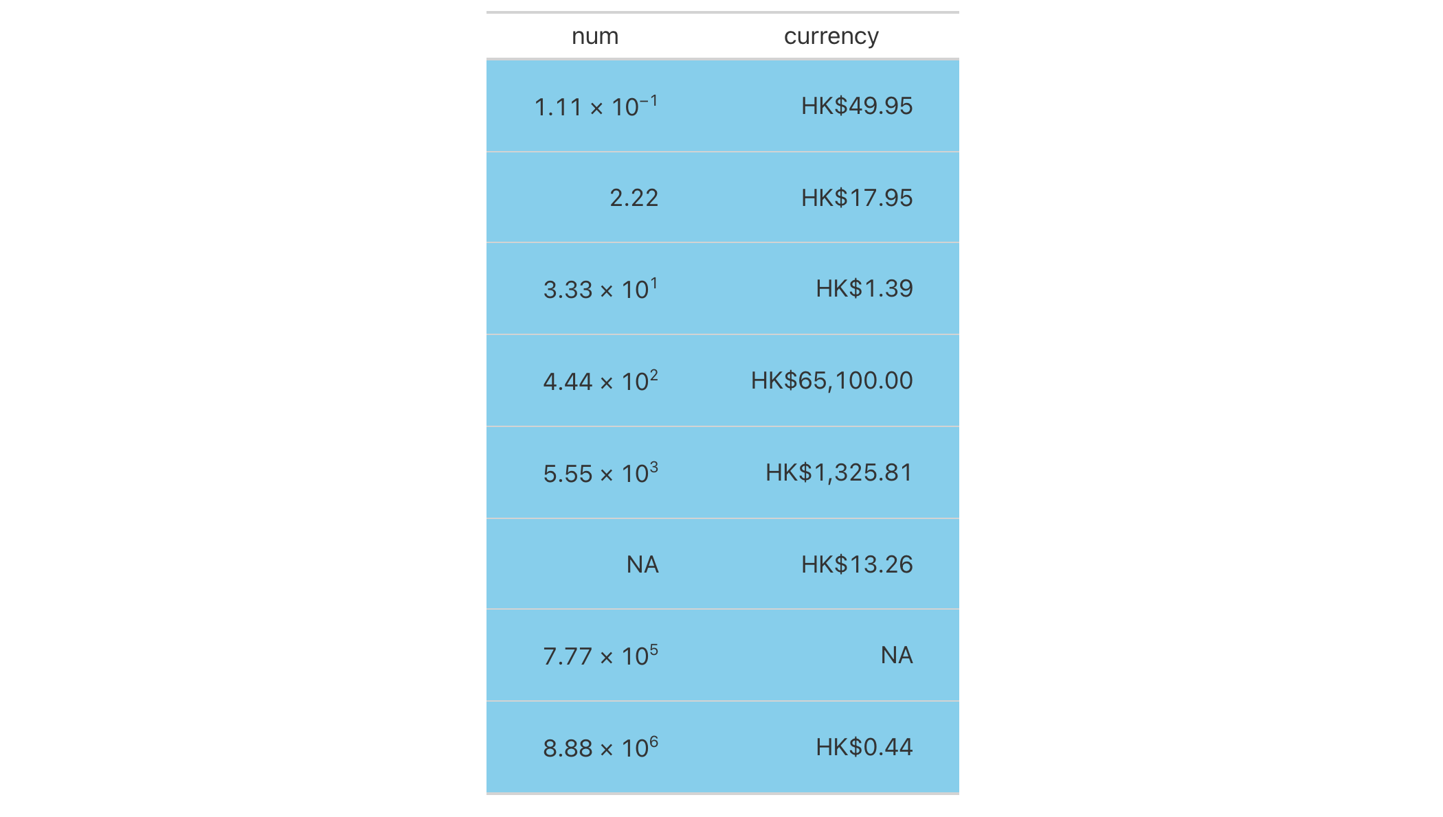
Function ID
10-14
Function Introduced
v0.2.2 (August 5, 2020)
See Also
Other table option functions:
opt_align_table_header(),
opt_all_caps(),
opt_footnote_marks(),
opt_footnote_order(),
opt_footnote_spec(),
opt_horizontal_padding(),
opt_interactive(),
opt_row_striping(),
opt_stylize(),
opt_table_font(),
opt_table_lines(),
opt_table_outline(),
opt_vertical_padding()
Option to modify the set of footnote marks
Description
Alter the footnote marks for any footnotes that may be present in the table.
Either a vector of marks can be provided (including Unicode characters), or,
a specific keyword could be used to signify a preset sequence. This function
serves as a shortcut for using tab_options(footnotes.marks = {marks})
Usage
opt_footnote_marks(data, marks = "numbers")opt_footnote_marks(data, marks = "numbers")
Arguments
data |
The gt table data object
This is the gt table object that is commonly created through use of the
|
marks |
Sequence of footnote marks
Either a character vector of length greater than 1 (that will represent the
series of marks) or a single keyword that represents a preset sequence of
marks. The valid keywords are: |
Value
An object of class gt_tbl.
Specification of footnote marks
We can supply a vector that will represent the series of marks. The series of
footnote marks is recycled when its usage goes beyond the length of the set.
At each cycle, the marks are simply doubled, tripled, and so on (e.g., * ->
** -> ***). The option exists for providing keywords for certain types of
footnote marks. The keywords are:
-
"numbers": numeric marks, they begin from 1 and these marks are not subject to recycling behavior -
"letters": minuscule alphabetic marks, internally uses thelettersvector which contains 26 lowercase letters of the Roman alphabet -
"LETTERS": majuscule alphabetic marks, using theLETTERSvector which has 26 uppercase letters of the Roman alphabet -
"standard": symbolic marks, four symbols in total -
"extended": symbolic marks, extends the standard set by adding two more symbols, making six
The symbolic marks are the: (1) Asterisk, (2) Dagger, (3) Double Dagger,
(4) Section Sign, (5) Double Vertical Line, and (6) Paragraph Sign; the
"standard" set has the first four, "extended" contains all.
Examples
Use a summarized version of the sza dataset to create a gt table,
adding three footnotes (with three calls of tab_footnote()). We can modify
the footnote marks to use with the opt_footnote_marks() function. With the
keyword "standard" we get four commonly-used typographic marks.
sza |>
dplyr::filter(latitude == 30) |>
dplyr::group_by(tst) |>
dplyr::summarize(
SZA.Max = if (
all(is.na(sza))) {
NA
} else {
max(sza, na.rm = TRUE)
},
SZA.Min = if (
all(is.na(sza))) {
NA
} else {
min(sza, na.rm = TRUE)
},
.groups = "drop"
) |>
gt(rowname_col = "tst") |>
tab_spanner_delim(delim = ".") |>
sub_missing(
columns = everything(),
missing_text = "90+"
) |>
tab_stubhead(label = "TST") |>
tab_footnote(
footnote = "True solar time.",
locations = cells_stubhead()
) |>
tab_footnote(
footnote = "Solar zenith angle.",
locations = cells_column_spanners(
spanners = "spanner-SZA.Max"
)
) |>
tab_footnote(
footnote = "The Lowest SZA.",
locations = cells_stub(rows = "1200")
) |>
opt_footnote_marks(marks = "standard")

Function ID
10-3
Function Introduced
v0.2.0.5 (March 31, 2020)
See Also
Other table option functions:
opt_align_table_header(),
opt_all_caps(),
opt_css(),
opt_footnote_order(),
opt_footnote_spec(),
opt_horizontal_padding(),
opt_interactive(),
opt_row_striping(),
opt_stylize(),
opt_table_font(),
opt_table_lines(),
opt_table_outline(),
opt_vertical_padding()
Option to modify the order of footnotes
Description
We can alter the order in which marked footnotes appear in relation to any unmarked footnotes in the footer section of the table. A single keyword is to be supplied and it will determine whether marked footnotes should appear: (1) before unmarked, (2) after unmarked, or (3) in call order.
Usage
opt_footnote_order(data, order = "marks_last")opt_footnote_order(data, order = "marks_last")
Arguments
data |
The gt table data object
This is the gt table object that is commonly created through use of the
|
order |
Method for ordering footnote marks
A keyword provided here will determine how marked footnotes will be
arranged in relation to unmarked footnotes. Use either: |
Value
An object of class gt_tbl.
Specification of footnote order
The keywords are:
-
"marks_last": marked footnotes should appear beneath unmarked in the table (default) -
"marks_first": marked footnotes should appear before unmarked in the table -
"preserve_order": footnotes will appear in the order they were specified intab_footnote()
Examples
Use a summarized version of the sza dataset to create a gt table,
adding three marked footnotes and one unmarked (with four calls of
tab_footnote()). We can modify the order of footnotes with the
opt_footnote_order() function.
sza |>
dplyr::filter(latitude == 30) |>
dplyr::group_by(tst) |>
dplyr::summarize(
SZA.Max = if (
all(is.na(sza))) {
NA
} else {
max(sza, na.rm = TRUE)
},
SZA.Min = if (
all(is.na(sza))) {
NA
} else {
min(sza, na.rm = TRUE)
},
.groups = "drop"
) |>
gt(rowname_col = "tst") |>
tab_spanner_delim(delim = ".") |>
sub_missing(
columns = everything(),
missing_text = "90+"
) |>
tab_stubhead(label = "TST") |>
tab_footnote(
footnote = "True solar time.",
locations = cells_stubhead()
) |>
tab_footnote(
footnote = "Solar zenith angle.",
locations = cells_column_spanners(
spanners = "spanner-SZA.Max"
)
) |>
tab_footnote(
footnote = "The Lowest SZA.",
locations = cells_stub(rows = "1200")
) |>
tab_footnote(
footnote = "Values calculated on the first of every month."
) |>
opt_footnote_order(order = "marks_first")
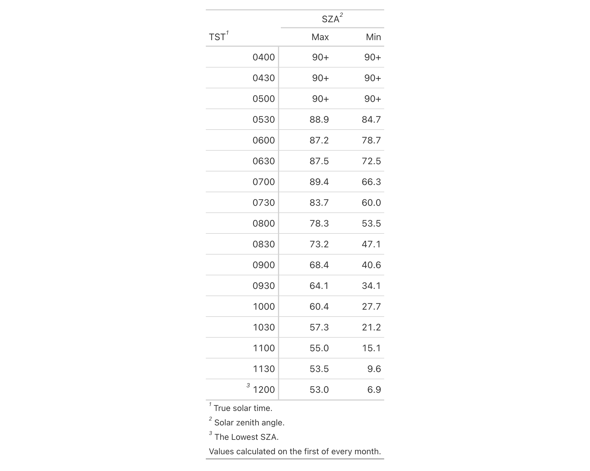
Function ID
10-5
Function Introduced
v0.1.1.9000 (September 22, 2025)
See Also
Other table option functions:
opt_align_table_header(),
opt_all_caps(),
opt_css(),
opt_footnote_marks(),
opt_footnote_spec(),
opt_horizontal_padding(),
opt_interactive(),
opt_row_striping(),
opt_stylize(),
opt_table_font(),
opt_table_lines(),
opt_table_outline(),
opt_vertical_padding()
Option to specify the formatting of footnote marks
Description
Modify the way footnote marks are formatted. This can be performed for those
footnote marks that alight to the targeted text in cells in various locations
in the table or the footnote marks that appear in the table footer. A simple
specification string can be provided for either or both types of marks in
opt_footnote_spec() . This function serves as a shortcut for using either
of tab_options(footnotes.spec_ref = {spec}) or
tab_options(footnotes.spec_ftr = {spec}).
Usage
opt_footnote_spec(data, spec_ref = NULL, spec_ftr = NULL)opt_footnote_spec(data, spec_ref = NULL, spec_ftr = NULL)
Arguments
data |
The gt table data object
This is the gt table object that is commonly created through use of the
|
spec_ref, spec_ftr
|
Specifications for formatting of footnote marks
Specification of the footnote marks when behaving as footnote references
and as marks in the footer section of the table. This is a string
containing spec characters. The default is the spec string |
Value
An object of class gt_tbl.
Specification rules for the formatting of footnote marks
A footnote spec consists of a string containing control characters for formatting. Not every type of formatting makes sense for footnote marks so the specification is purposefully constrained to the following:
-
as superscript text (with the
"^"control character) or regular-sized text residing on the baseline -
bold text (with
"b"), italicized text (with"i"), or unstyled text (don't use either of the"b"or"i"control characters) -
enclosure in parentheses (use
"("/")") or square brackets (with"["/"]") -
a period following the mark (using
"."); this is most commonly used in the table footer
With the aforementioned control characters we could, for instance, format
the footnote marks to be superscript text in bold type with "^b". We might
want the marks in the footer to be regular-sized text in parentheses, so the
spec could be either "()" or "(x)" (you can optionally use "x" as a
helpful placeholder for the marks).
Examples
Use a modified version of sp500 the dataset to create a gt table with
row labels. We'll add two footnotes using the tab_footnote() function. We
can call opt_footnote_spec() to specify that the marks of the footnote
reference should be superscripts in bold, and, the marks in the footer
section should be enclosed in parentheses.
sp500 |>
dplyr::filter(date >= "1987-10-14" & date <= "1987-10-25") |>
dplyr::select(date, open, close, volume) |>
dplyr::mutate(difference = close - open) |>
dplyr::mutate(change = (close - open) / open) |>
dplyr::mutate(day = vec_fmt_datetime(date, format = "E")) |>
dplyr::arrange(-dplyr::row_number()) |>
gt(rowname_col = "date") |>
fmt_currency() |>
fmt_number(columns = volume, suffixing = TRUE) |>
fmt_percent(columns = change) |>
cols_move_to_start(columns = day) |>
cols_width(
stub() ~ px(130),
day ~ px(50),
everything() ~ px(100)
) |>
tab_footnote(
footnote = "Commerce report on trade deficit.",
locations = cells_stub(rows = 1)
) |>
tab_footnote(
footnote = "Black Monday market crash, representing the greatest
one-day percentage decline in U.S. stock market history.",
locations = cells_body(columns = change, rows = change < -0.15)
) |>
opt_footnote_spec(spec_ref = "^xb", spec_ftr = "(x)")

Function ID
10-4
Function Introduced
v0.9.0 (Mar 31, 2023)
See Also
Other table option functions:
opt_align_table_header(),
opt_all_caps(),
opt_css(),
opt_footnote_marks(),
opt_footnote_order(),
opt_horizontal_padding(),
opt_interactive(),
opt_row_striping(),
opt_stylize(),
opt_table_font(),
opt_table_lines(),
opt_table_outline(),
opt_vertical_padding()
Option to expand or contract horizontal padding
Description
Increase or decrease the horizontal padding throughout all locations of a
gt table by use of a scale factor, which here is defined by a real
number between 0 and 3. This function serves as a shortcut for setting
the following eight options in tab_options():
-
heading.padding.horizontal -
column_labels.padding.horizontal -
data_row.padding.horizontal -
row_group.padding.horizontal -
summary_row.padding.horizontal -
grand_summary_row.padding.horizontal -
footnotes.padding.horizontal -
source_notes.padding.horizontal
Usage
opt_horizontal_padding(data, scale = 1)opt_horizontal_padding(data, scale = 1)
Arguments
data |
The gt table data object
This is the gt table object that is commonly created through use of the
|
scale |
Scale factor
A scale factor by which the horizontal padding will be adjusted. Must be a
number between |
Value
An object of class gt_tbl.
Examples
Use the exibble dataset to create a gt table with a number of table
parts added (using functions like summary_rows(), grand_summary_rows(),
and more). Following that, we'll increase the amount of horizontal padding
across the entire table with opt_horizontal_padding(). Using a scale
value of 3 (up from the default of 1) means the horizontal space will
be greatly increased, resulting in a more spacious table.
exibble |>
gt(rowname_col = "row", groupname_col = "group") |>
summary_rows(
groups = "grp_a",
columns = c(num, currency),
fns = c("min", "max")
) |>
grand_summary_rows(
columns = currency,
fns = total ~ sum(., na.rm = TRUE)
) |>
tab_source_note(source_note = "This is a source note.") |>
tab_footnote(
footnote = "This is a footnote.",
locations = cells_body(columns = 1, rows = 1)
) |>
tab_header(
title = "The title of the table",
subtitle = "The table's subtitle"
) |>
opt_horizontal_padding(scale = 3)
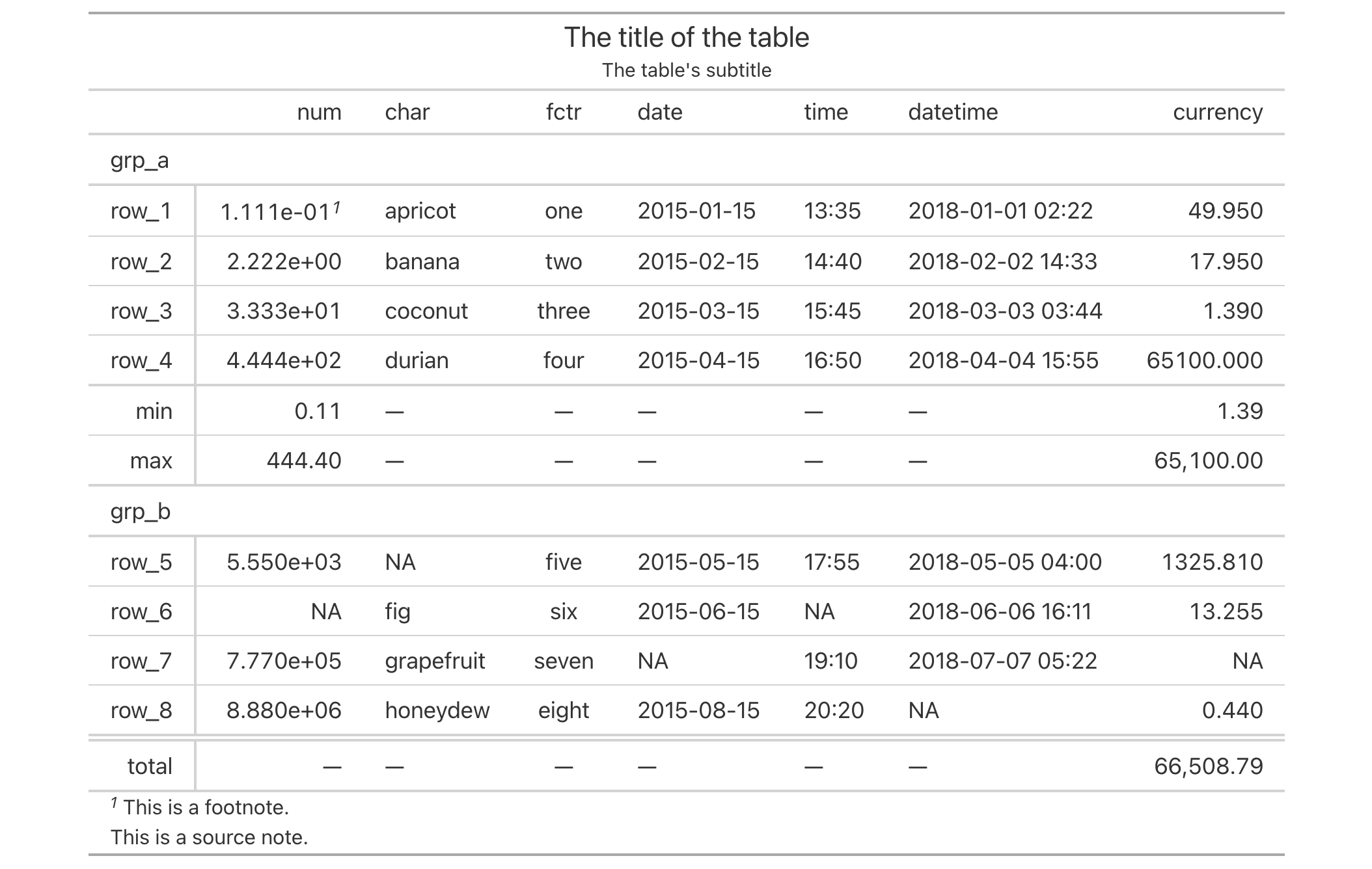
Function ID
10-9
Function Introduced
v0.4.0 (February 15, 2022)
See Also
Other table option functions:
opt_align_table_header(),
opt_all_caps(),
opt_css(),
opt_footnote_marks(),
opt_footnote_order(),
opt_footnote_spec(),
opt_interactive(),
opt_row_striping(),
opt_stylize(),
opt_table_font(),
opt_table_lines(),
opt_table_outline(),
opt_vertical_padding()
Option to put interactive elements in an HTML table
Description
By default, a gt table rendered as HTML will essentially be a 'static'
table. However, we can make it 'interactive' and configure those interactive
HTML options through the opt_interactive() function. Making an HTML table
interactive entails the enabling of controls for pagination, global search,
filtering, sorting, and more.
This function serves as a shortcut for setting the following options in
tab_options():
-
ihtml.active -
ihtml.use_pagination -
ihtml.use_pagination_info -
ihtml.use_sorting -
ihtml.use_search -
ihtml.use_filters -
ihtml.use_resizers -
ihtml.use_highlight -
ihtml.use_compact_mode -
ihtml.use_page_size_select -
ihtml.page_size_default -
ihtml.page_size_values -
ihtml.pagination_type -
ihtml.height -
ihtml.selection_mode
Usage
opt_interactive( data, active = TRUE, use_pagination = TRUE, use_pagination_info = TRUE, use_sorting = TRUE, use_search = FALSE, use_filters = FALSE, use_resizers = FALSE, use_highlight = FALSE, use_compact_mode = FALSE, use_text_wrapping = TRUE, use_page_size_select = FALSE, page_size_default = 10, page_size_values = c(10, 25, 50, 100), pagination_type = c("numbers", "jump", "simple"), height = "auto", selection_mode = NULL )opt_interactive( data, active = TRUE, use_pagination = TRUE, use_pagination_info = TRUE, use_sorting = TRUE, use_search = FALSE, use_filters = FALSE, use_resizers = FALSE, use_highlight = FALSE, use_compact_mode = FALSE, use_text_wrapping = TRUE, use_page_size_select = FALSE, page_size_default = 10, page_size_values = c(10, 25, 50, 100), pagination_type = c("numbers", "jump", "simple"), height = "auto", selection_mode = NULL )
Arguments
data |
The gt table data object
This is the gt table object that is commonly created through use of the
|
active |
Display interactive HTML table
The |
use_pagination |
Display pagination controls
This is the option for using pagination controls (below the table body). By
default, this is |
use_pagination_info |
Display pagination info
If |
use_sorting |
Provide column sorting controls
This option provides controls for sorting column values. By default, this
is |
use_search |
Provide a global search field
The |
use_filters |
Display filtering fields
The |
use_resizers |
Allow column resizing
This option allows for the interactive resizing of columns. By default,
this is |
use_highlight |
Enable row highlighting on hover
The |
use_compact_mode |
Use compact mode
To reduce vertical padding and thus make the table consume less vertical
space the |
use_text_wrapping |
Use text wrapping
The |
use_page_size_select |
Allow for page size selection
The |
page_size_default |
Change the default page size
The default page size (initially set as |
page_size_values |
Set of page-size values
By default, this is the vector |
pagination_type |
Change pagination mode
When using pagination the |
height |
Height of interactive HTML table Height of the table in pixels. Defaults to |
selection_mode |
Allow row selection
The |
Value
An object of class gt_tbl.
Examples
Use select columns from the towny dataset to create a gt table with a
header (through tab_header()) and a source note (through
tab_source_note()). Next, we will add interactive HTML features (and
otherwise activate interactive HTML mode) through opt_interactive(). It'll
just be the default set of interactive options.
towny |>
dplyr::select(name, census_div, starts_with("population")) |>
gt() |>
fmt_integer() |>
cols_label_with(fn = function(x) sub("population_", "", x)) |>
cols_width(
name ~ px(200),
census_div ~ px(200)
) |>
tab_header(
title = "Populations of Municipalities",
subtitle = "Census values from 1996 to 2021."
) |>
tab_source_note(source_note = md("Data taken from the `towny` dataset.")) |>
opt_interactive()

Interactive tables can have styled body cells. Here, we use the gtcars
dataset to create an interactive gt table. Using tab_style() and
data_color() we can flexibly style body cells throughout the table.
gtcars |>
gt() |>
cols_width(everything() ~ px(130)) |>
tab_style(
style = cell_fill(color = "gray95"),
locations = cells_body(columns = c(mfr, model))
) |>
data_color(
columns = c(starts_with("hp"), starts_with("trq")),
method = "numeric",
palette = "viridis"
) |>
cols_hide(columns = trim) |>
opt_interactive()

Function ID
10-2
Function Introduced
v0.9.0 (Mar 31, 2023)
See Also
Other table option functions:
opt_align_table_header(),
opt_all_caps(),
opt_css(),
opt_footnote_marks(),
opt_footnote_order(),
opt_footnote_spec(),
opt_horizontal_padding(),
opt_row_striping(),
opt_stylize(),
opt_table_font(),
opt_table_lines(),
opt_table_outline(),
opt_vertical_padding()
Option to add or remove row striping
Description
By default, a gt table does not have row striping enabled. However, this
function allows us to easily enable or disable striped rows in the table
body. This function serves as a convenient shortcut for
<gt_tbl> |> tab_options(row.striping.include_table_body = TRUE|FALSE).
Usage
opt_row_striping(data, row_striping = TRUE)opt_row_striping(data, row_striping = TRUE)
Arguments
data |
The gt table data object
This is the gt table object that is commonly created through use of the
|
row_striping |
Use alternating row stripes
A logical value to indicate whether row striping should be added or removed. |
Value
An object of class gt_tbl.
Examples
Use the exibble dataset to create a gt table with a number of table
parts added (using functions like summary_rows(), grand_summary_rows(),
and more). Following that, we'll add row striping to every second row with
opt_row_striping().
exibble |>
gt(rowname_col = "row", groupname_col = "group") |>
summary_rows(
groups = "grp_a",
columns = c(num, currency),
fns = c("min", "max")
) |>
grand_summary_rows(
columns = currency,
fns = total ~ sum(., na.rm = TRUE)
) |>
tab_source_note(source_note = "This is a source note.") |>
tab_footnote(
footnote = "This is a footnote.",
locations = cells_body(columns = 1, rows = 1)
) |>
tab_header(
title = "The title of the table",
subtitle = "The table's subtitle"
) |>
opt_row_striping()
Function ID
10-6
Function Introduced
v0.2.0.5 (March 31, 2020)
See Also
Other table option functions:
opt_align_table_header(),
opt_all_caps(),
opt_css(),
opt_footnote_marks(),
opt_footnote_order(),
opt_footnote_spec(),
opt_horizontal_padding(),
opt_interactive(),
opt_stylize(),
opt_table_font(),
opt_table_lines(),
opt_table_outline(),
opt_vertical_padding()
Stylize your table with a colorful look
Description
With opt_stylize() you can quickly style your gt table with a carefully
curated set of background colors, line colors, and line styles. There are six
styles to choose from and they largely vary in the extent of coloring applied
to different table locations. Some have table borders applied, some apply
darker colors to the table stub and summary sections, and, some even have
vertical lines. In addition to choosing a style preset, there are six
color variations that each use a range of five color tints. Each of the
color tints have been fine-tuned to maximize the contrast between text and
its background. There are 36 combinations of style and color to choose
from.
Usage
opt_stylize(data, style = 1, color = "blue", add_row_striping = TRUE)opt_stylize(data, style = 1, color = "blue", add_row_striping = TRUE)
Arguments
data |
The gt table data object
This is the gt table object that is commonly created through use of the
|
style |
Table style
Six numbered styles are available. Simply provide a number from |
color |
Color variation
There are six color variations: |
add_row_striping |
Allow row striping
An option to enable row striping in the table body for the |
Value
an object of class gt_tbl.
Examples
Use exibble to create a gt table with a number of table parts added.
Then, use opt_stylize() to give the table some additional style
(using the "cyan" color variation and style number 6).
exibble |>
gt(rowname_col = "row", groupname_col = "group") |>
summary_rows(
groups = "grp_a",
columns = c(num, currency),
fns = c("min", "max")
) |>
grand_summary_rows(
columns = currency,
fns = total ~ sum(., na.rm = TRUE)
) |>
tab_source_note(source_note = "This is a source note.") |>
tab_footnote(
footnote = "This is a footnote.",
locations = cells_body(columns = 1, rows = 1)
) |>
tab_header(
title = "The title of the table",
subtitle = "The table's subtitle"
) |>
opt_stylize(style = 6, color = "cyan")
Function ID
10-1
Function Introduced
v0.7.0 (Aug 25, 2022)
See Also
Other table option functions:
opt_align_table_header(),
opt_all_caps(),
opt_css(),
opt_footnote_marks(),
opt_footnote_order(),
opt_footnote_spec(),
opt_horizontal_padding(),
opt_interactive(),
opt_row_striping(),
opt_table_font(),
opt_table_lines(),
opt_table_outline(),
opt_vertical_padding()
Options to define font choices for the entire table
Description
opt_table_font() makes it possible to define fonts used for an entire
gt table. Any font names supplied in font will (by default, with
add = TRUE) be placed before the names present in the existing font stack
(i.e., they will take precedence). You can choose to base the font stack on
those provided by system_fonts() by providing a valid keyword for a themed
set and optionally prepending font values to that.
Take note that you could still have entirely different fonts in specific
locations of the table. For that you would need to use tab_style() or
tab_style_body() in conjunction with cell_text().
Usage
opt_table_font( data, font = NULL, stack = NULL, size = NULL, weight = NULL, style = NULL, color = NULL, add = TRUE )opt_table_font( data, font = NULL, stack = NULL, size = NULL, weight = NULL, style = NULL, color = NULL, add = TRUE )
Arguments
data |
The gt table data object
This is the gt table object that is commonly created through use of the
|
font |
Default table fonts
One or more font names available as system or web fonts. These can be
combined with a |
stack |
Name of font stack
A name that is representative of a font stack (obtained via internally via
the |
size |
Text size
The text size for the entire table can be set by providing a |
weight |
Text weight
Option to set the weight of the font. Can be a text-based keyword such as
|
style |
Text style
An option to modify the text style. Can be one of either |
color |
Text color
The |
add |
Add to existing fonts
Should fonts be added to the beginning of any already-defined fonts for the
table? By default, this is |
Value
An object of class gt_tbl.
Possibilities for the font argument
We have the option to supply one or more font names for the font argument.
They can be enclosed in c() or a list(). You can generate this list or
vector with a combination of font names, and you can freely use
google_font(), default_fonts(), and system_fonts() to help compose
your font family.
Possibilities for the stack argument
There are several themed font stacks available via the system_fonts()
helper function. That function can be used to generate all or a segment of a
vector supplied to the font argument. However, using the stack argument
with one of the 15 keywords for the font stacks available in
system_fonts(), we could be sure that the typeface class will work across
multiple computer systems. Any of the following keywords can be used:
-
"system-ui" -
"transitional" -
"old-style" -
"humanist" -
"geometric-humanist" -
"classical-humanist" -
"neo-grotesque" -
"monospace-slab-serif" -
"monospace-code" -
"industrial" -
"rounded-sans" -
"slab-serif" -
"antique" -
"didone" -
"handwritten"
Examples
Use a subset of the sp500 dataset to create a small gt table. We'll
use fmt_currency() to display a dollar sign for the first row of monetary
values. The "Merriweather" font (from Google Fonts, via google_font())
with two system font fallbacks ("Cochin" and the generic "serif").
sp500 |>
dplyr::slice(1:10) |>
dplyr::select(-volume, -adj_close) |>
gt() |>
fmt_currency(
rows = 1,
use_seps = FALSE
) |>
opt_table_font(
font = list(
google_font(name = "Merriweather"),
"Cochin", "serif"
)
)
With the sza dataset we'll create a two-column, eleven-row table. Within
opt_table_font(), the stack argument will be supplied with the
"rounded-sans" font stack. This sets up a family of fonts with rounded,
curved letterforms that should be locally available in different computing
environments.
sza |>
dplyr::filter(
latitude == 20 &
month == "jan" &
!is.na(sza)
) |>
dplyr::select(-latitude, -month) |>
gt() |>
opt_table_font(stack = "rounded-sans") |>
opt_all_caps()
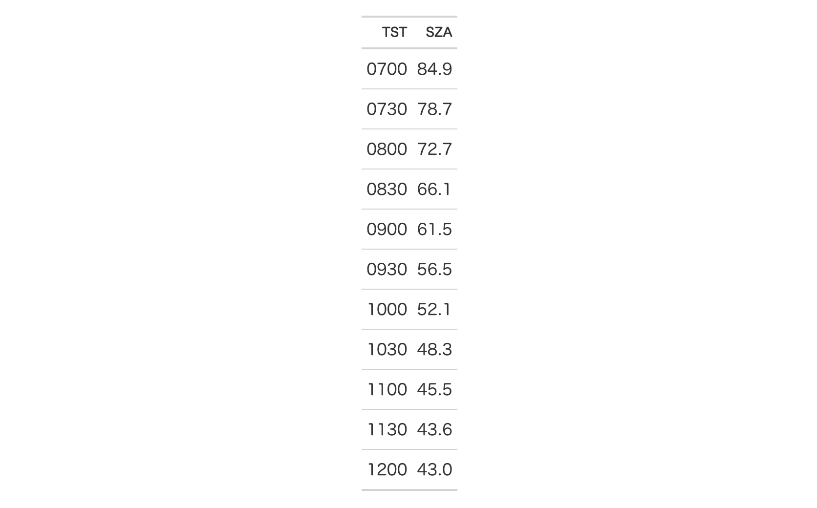
Function ID
10-13
Function Introduced
v0.2.2 (August 5, 2020)
See Also
Other table option functions:
opt_align_table_header(),
opt_all_caps(),
opt_css(),
opt_footnote_marks(),
opt_footnote_order(),
opt_footnote_spec(),
opt_horizontal_padding(),
opt_interactive(),
opt_row_striping(),
opt_stylize(),
opt_table_lines(),
opt_table_outline(),
opt_vertical_padding()
Option to set table lines to different extents
Description
opt_table_lines() sets table lines in one of three possible ways:
(1) all possible table lines drawn ("all"), (2) no table lines at all
("none"), and (3) resetting to the default line styles ("default"). This
is great if you want to start off with lots of lines and subtract just a few
of them with tab_options() or tab_style(). Or, use it to start with a
completely lineless table, adding individual lines as needed.
Usage
opt_table_lines(data, extent = c("all", "none", "default"))opt_table_lines(data, extent = c("all", "none", "default"))
Arguments
data |
The gt table data object
This is the gt table object that is commonly created through use of the
|
extent |
Extent of lines added
The extent to which lines will be visible in the table. Options are
|
Value
An object of class gt_tbl.
Examples
Use the exibble dataset to create a gt table with a number of table
parts added (using functions like summary_rows(), grand_summary_rows(),
and more). Following that, we'll use the opt_table_lines() function to
generate lines everywhere there can possibly be lines (the default for the
extent argument is "all").
exibble |>
gt(rowname_col = "row", groupname_col = "group") |>
summary_rows(
groups = "grp_a",
columns = c(num, currency),
fns = c("min", "max")
) |>
grand_summary_rows(
columns = currency,
fns = total ~ sum(., na.rm = TRUE)
) |>
tab_source_note(source_note = "This is a source note.") |>
tab_footnote(
footnote = "This is a footnote.",
locations = cells_body(columns = 1, rows = 1)
) |>
tab_header(
title = "The title of the table",
subtitle = "The table's subtitle"
) |>
opt_table_lines()
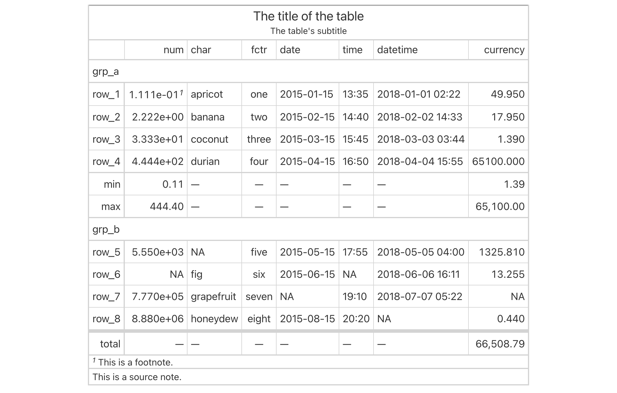
Function ID
10-11
Function Introduced
v0.2.0.5 (March 31, 2020)
See Also
Other table option functions:
opt_align_table_header(),
opt_all_caps(),
opt_css(),
opt_footnote_marks(),
opt_footnote_order(),
opt_footnote_spec(),
opt_horizontal_padding(),
opt_interactive(),
opt_row_striping(),
opt_stylize(),
opt_table_font(),
opt_table_outline(),
opt_vertical_padding()
Option to wrap an outline around the entire table
Description
This function puts an outline of consistent style, width, and color
around the entire table. It'll write over any existing outside lines so long
as the width is larger that of the existing lines. The default value of
style ("solid") will draw a solid outline, whereas a value of "none"
will remove any present outline.
Usage
opt_table_outline(data, style = "solid", width = px(3), color = "#D3D3D3")opt_table_outline(data, style = "solid", width = px(3), color = "#D3D3D3")
Arguments
data |
The gt table data object
This is the gt table object that is commonly created through use of the
|
style |
Outline style property
The style property for the table outline. By default, this is |
width |
Outline width value
The width property for the table outline. By default, this is |
color |
Color of outline
The color of the table outline. By default, this is |
Value
An object of class gt_tbl.
Examples
Use the exibble dataset to create a gt table with a number of table
parts added (using functions like summary_rows(), grand_summary_rows(),
and more). Following that, let's make it so that we have an outline wrap
around the entire table by using the opt_table_outline() function.
tab_1 <-
exibble |>
gt(rowname_col = "row", groupname_col = "group") |>
summary_rows(
groups = "grp_a",
columns = c(num, currency),
fns = c("min", "max")
) |>
grand_summary_rows(
columns = currency,
fns = total ~ sum(., na.rm = TRUE)
) |>
tab_source_note(source_note = "This is a source note.") |>
tab_footnote(
footnote = "This is a footnote.",
locations = cells_body(columns = 1, rows = 1)
) |>
tab_header(
title = "The title of the table",
subtitle = "The table's subtitle"
) |>
opt_table_outline()
tab_1

Remove the table outline with the style = "none" option.
tab_1 |> opt_table_outline(style = "none")

Function ID
10-12
Function Introduced
v0.2.0.5 (March 31, 2020)
See Also
Other table option functions:
opt_align_table_header(),
opt_all_caps(),
opt_css(),
opt_footnote_marks(),
opt_footnote_order(),
opt_footnote_spec(),
opt_horizontal_padding(),
opt_interactive(),
opt_row_striping(),
opt_stylize(),
opt_table_font(),
opt_table_lines(),
opt_vertical_padding()
Option to expand or contract vertical padding
Description
Increase or decrease the vertical padding throughout all locations of a
gt table by use of a scale factor, which here is defined by a real
number between 0 and 3. This function serves as a shortcut for setting
the following eight options in tab_options():
-
heading.padding -
column_labels.padding -
data_row.padding -
row_group.padding -
summary_row.padding -
grand_summary_row.padding -
footnotes.padding -
source_notes.padding
Usage
opt_vertical_padding(data, scale = 1)opt_vertical_padding(data, scale = 1)
Arguments
data |
The gt table data object
This is the gt table object that is commonly created through use of the
|
scale |
Scale factor
A scale factor by which the vertical padding will be adjusted. Must be a
number between |
Value
An object of class gt_tbl.
Examples
Use the exibble dataset to create a gt table with a number of table
parts added (using functions like summary_rows(), grand_summary_rows(),
and more). Following that, we'll lessen the amount of vertical padding across
the entire table with opt_vertical_padding(). Using a scale value of
0.25 (down from the default of 1) means the vertical space will be
greatly reduced, resulting in a more compact table.
exibble |>
gt(rowname_col = "row", groupname_col = "group") |>
summary_rows(
groups = "grp_a",
columns = c(num, currency),
fns = c("min", "max")
) |>
grand_summary_rows(
columns = currency,
fns = total ~ sum(., na.rm = TRUE)
) |>
tab_source_note(source_note = "This is a source note.") |>
tab_footnote(
footnote = "This is a footnote.",
locations = cells_body(columns = 1, rows = 1)
) |>
tab_header(
title = "The title of the table",
subtitle = "The table's subtitle"
) |>
opt_vertical_padding(scale = 0.25)
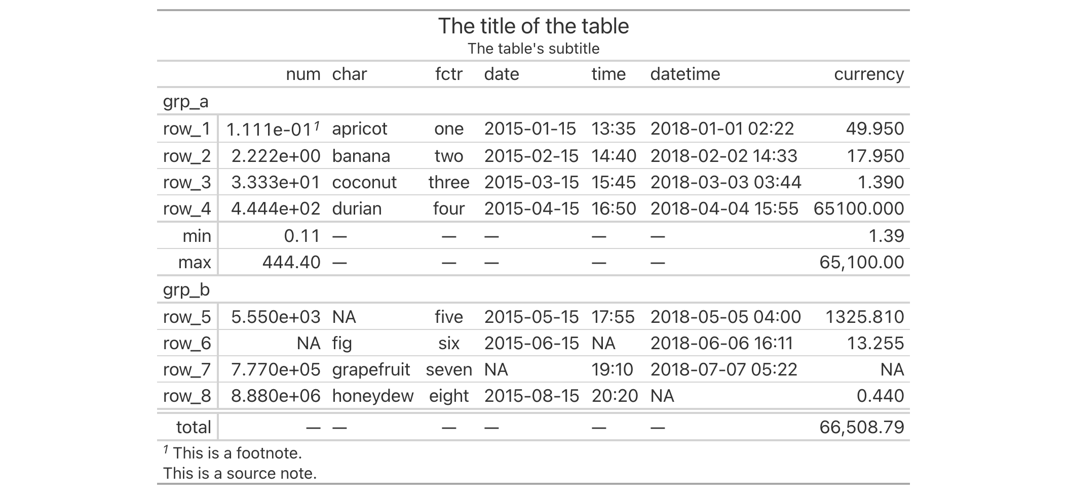
Function ID
10-8
Function Introduced
v0.4.0 (February 15, 2022)
See Also
Other table option functions:
opt_align_table_header(),
opt_all_caps(),
opt_css(),
opt_footnote_marks(),
opt_footnote_order(),
opt_footnote_spec(),
opt_horizontal_padding(),
opt_interactive(),
opt_row_striping(),
opt_stylize(),
opt_table_font(),
opt_table_lines(),
opt_table_outline()
Helper for providing a numeric value as percentage
Description
A percentage value acts as a length value that is relative to an initial
state. For instance an 80 percent value for something will size the target
to 80 percent the size of its 'previous' value. This type of sizing is
useful for sizing up or down a length value with an intuitive measure. This
helper function can be used for the setting of font sizes (e.g., in
cell_text()) and altering the thicknesses of lines (e.g., in
cell_borders()). Should a more exact definition of size be required, the
analogous helper function pct() will be more useful.
Usage
pct(x)pct(x)
Arguments
x |
Numeric value in percent
The numeric value to format as a string percentage for some |
Value
A character vector with a single value in percentage units.
Examples
Use the exibble dataset to create a gt table. Inside of the
cell_text() call (which is itself inside of tab_style()), we'll use the
pct() helper function to define the font size for the column labels as a
percentage value.
exibble |>
gt() |>
tab_style(
style = cell_text(size = pct(75)),
locations = cells_column_labels()
)
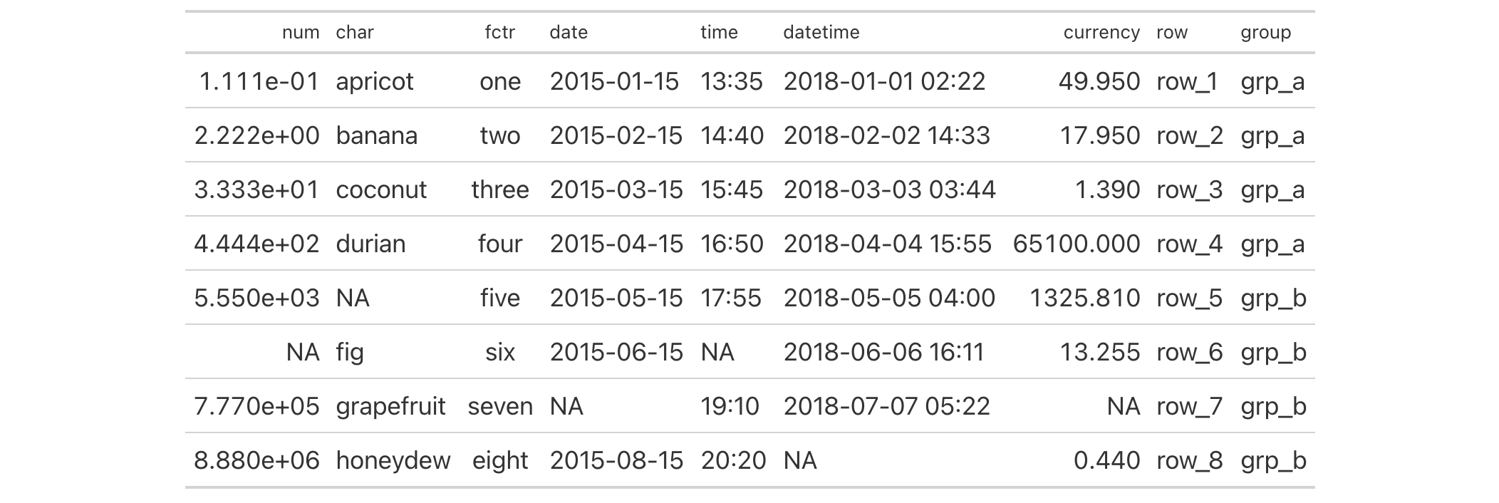
Function ID
8-4
Function Introduced
v0.2.0.5 (March 31, 2020)
See Also
Other helper functions:
adjust_luminance(),
cell_borders(),
cell_fill(),
cell_text(),
currency(),
default_fonts(),
escape_latex(),
from_column(),
google_font(),
gt_latex_dependencies(),
html(),
latex(),
md(),
nanoplot_options(),
px(),
random_id(),
row_group(),
stub(),
system_fonts(),
unit_conversion()
A table of personal information for people all over the world
Description
The peeps dataset contains records for one hundred people residing in ten
different countries. Each person in the table has address information along
with their email address and phone number. There are also personal
characteristics like date of birth, height, and weight. This data has been
synthesized, and so the names within the table have not been taken or based
on individuals in real life. The street addresses were generated from actual
street names within real geographic localities, however, the street numbers
were assigned randomly from a constrained number set. While these records do
not relate to real people, efforts were made to make the data as realistic as
possible.
Usage
peepspeeps
Format
A tibble with 100 rows and 14 variables:
- name_given, name_family
-
The given and family name of individual.
- address
-
The street address of the individual.
- city
-
The name of the city or locality in which the individual resides.
- state_prov
-
The state or province associated with the
cityandaddress. This isNAfor individuals residing in countries where subdivision data is not needed for generating a valid mailing address. - postcode
-
The post code associated with the
cityandaddress. - country
-
The 3-letter ISO 3166-1 country code representative of the individual's country.
- email_addr
-
The individual's email address.
- phone_number, country_code
-
The individual's phone number and the country code associated with the phone number.
- gender
-
The gender of the individual.
- dob
-
The individual's date of birth (DOB) in the ISO 8601 form of
YYYY-MM-DD. - height_cm, weight_kg
-
The height and weight of the individual in centimeters (cm) and kilograms (kg), respectively.
Dataset ID and Badge
DATA-8

Dataset Introduced
v0.11.0 (July 9, 2024)
See Also
Other datasets:
constants,
countrypops,
exibble,
films,
gibraltar,
gtcars,
illness,
metro,
nuclides,
photolysis,
pizzaplace,
reactions,
rx_addv,
rx_adsl,
sp500,
sza,
towny
Examples
dplyr::glimpse(peeps)dplyr::glimpse(peeps)
Data on photolysis rates for gas-phase organic compounds
Description
The photolysis dataset contains numerical values for describing the
photolytic degradation pathways of 25 compounds of relevance in atmospheric
chemistry. Many volatile organic compounds (VOCs) are emitted in substantial
quantities from both biogenic and anthropogenic sources, and they can have a
major influence on the chemistry of the lower atmosphere. A portion of these
can be transformed into other VOCs via the energy provided from light.
In order to realistically predict the composition of the atmosphere and how
it evolves over time, we need accurate estimates of photolysis rates. The
data provided here in photolysis allows for computations of photolysis
rates (J, having units of s^-1) as a function of the solar zenith angle
(SZA). Having such values is essential when deploying atmospheric chemistry
models.
Usage
photolysisphotolysis
Format
A tibble with 34 rows and 10 variables:
- compd_name
-
The name of the primary compound undergoing photolysis.
- cmpd_formula
-
The chemical formula of the compound.
- products
-
A product pathway for the photolysis of the compound.
- type
-
The type of organic compound undergoing photolysis.
- l, m, n
-
The parameter values given in the
l,m, andncolumns can be used to calculate the photolysis rate (J) as a function of the solar zenith angle (X, in radians) through the expression:J = l * cos(X)^m * exp(-n * sec(X)). - quantum_yield
-
In the context of photolysis reactions, this is the efficiency of a given photolytic reaction. In other words, it's the number of product molecules formed over the number of photons absorbed.
- wavelength_nm, sigma_298_cm2
-
The
wavelength_nmandsigma_298_cm2columns provide photoabsorption data for the compound undergoing photolysis. The values inwavelength_nmprovide the wavelength of light in nanometer units; thesigma_298_cm2values are paired with thewavelength_nmvalues and they are in units ofcm^2 molecule^-1.
Dataset ID and Badge
DATA-15

Dataset Introduced
v0.11.0 (July 9, 2024)
See Also
Other datasets:
constants,
countrypops,
exibble,
films,
gibraltar,
gtcars,
illness,
metro,
nuclides,
peeps,
pizzaplace,
reactions,
rx_addv,
rx_adsl,
sp500,
sza,
towny
Examples
dplyr::glimpse(photolysis)dplyr::glimpse(photolysis)
A year of pizza sales from a pizza place
Description
A synthetic dataset that describes pizza sales for a pizza place somewhere in
the US. While the contents are artificial, the ingredients used to make the
pizzas are far from it. There are 32 different pizzas that fall into 4
different categories: "classic" (classic pizzas: 'You probably had one like
it before, but never like this!'), "chicken" (pizzas with chicken as a
major ingredient: 'Try the Southwest Chicken Pizza! You'll love it!'),
"supreme" (pizzas that try a little harder: 'My Soppressata pizza uses only
the finest salami from my personal salumist!'), and, "veggie" (pizzas
without any meats whatsoever: 'My Five Cheese pizza has so many cheeses, I
can only offer it in Large Size!').
Usage
pizzaplacepizzaplace
Format
A tibble with 49,574 rows and 7 variables:
- id
-
The ID for the order, which consists of one or more pizzas at a given
dateandtime. - date
-
A character representation of the order date, expressed in the ISO 8601 date format (
YYYY-MM-DD). - time
-
A character representation of the order time, expressed as a 24-hour time the ISO 8601 extended time format (
HH:MM:SS). - name
-
The short name for the pizza.
- size
-
The size of the pizza, which can either be
"S","M","L","XL"(rare!), or"XXL"(even rarer!); most pizzas are available in the"S","M", and"L"sizes but exceptions apply. - type
-
The category or type of pizza, which can either be
"classic","chicken","supreme", or"veggie". - price
-
The price of the pizza and the amount that it sold for (in USD).
Details
Each pizza in the dataset is identified by a short name. The following
listings provide the full names of each pizza and their main ingredients.
Classic Pizzas:
-
"classic_dlx": The Classic Deluxe Pizza (Pepperoni, Mushrooms, Red Onions, Red Peppers, Bacon) -
"big_meat": The Big Meat Pizza (Bacon, Pepperoni, Italian Sausage, Chorizo Sausage) -
"pepperoni": The Pepperoni Pizza (Mozzarella Cheese, Pepperoni) -
"hawaiian": The Hawaiian Pizza (Sliced Ham, Pineapple, Mozzarella Cheese) -
"pep_msh_pep": The Pepperoni, Mushroom, and Peppers Pizza (Pepperoni, Mushrooms, and Green Peppers) -
"ital_cpcllo": The Italian Capocollo Pizza (Capocollo, Red Peppers, Tomatoes, Goat Cheese, Garlic, Oregano) -
"napolitana": The Napolitana Pizza (Tomatoes, Anchovies, Green Olives, Red Onions, Garlic) -
"the_greek": The Greek Pizza (Kalamata Olives, Feta Cheese, Tomatoes, Garlic, Beef Chuck Roast, Red Onions)
Chicken Pizzas:
-
"thai_ckn": The Thai Chicken Pizza (Chicken, Pineapple, Tomatoes, Red Peppers, Thai Sweet Chilli Sauce) -
"bbq_ckn": The Barbecue Chicken Pizza (Barbecued Chicken, Red Peppers, Green Peppers, Tomatoes, Red Onions, Barbecue Sauce) -
"southw_ckn": The Southwest Chicken Pizza (Chicken, Tomatoes, Red Peppers, Red Onions, Jalapeno Peppers, Corn, Cilantro, Chipotle Sauce) -
"cali_ckn": The California Chicken Pizza (Chicken, Artichoke, Spinach, Garlic, Jalapeno Peppers, Fontina Cheese, Gouda Cheese) -
"ckn_pesto": The Chicken Pesto Pizza (Chicken, Tomatoes, Red Peppers, Spinach, Garlic, Pesto Sauce) -
"ckn_alfredo": The Chicken Alfredo Pizza (Chicken, Red Onions, Red Peppers, Mushrooms, Asiago Cheese, Alfredo Sauce)
Supreme Pizzas:
-
"brie_carre": The Brie Carre Pizza (Brie Carre Cheese, Prosciutto, Caramelized Onions, Pears, Thyme, Garlic) -
"calabrese": The Calabrese Pizza ('Nduja Salami, Pancetta, Tomatoes, Red Onions, Friggitello Peppers, Garlic) -
"soppressata": The Soppressata Pizza (Soppressata Salami, Fontina Cheese, Mozzarella Cheese, Mushrooms, Garlic) -
"sicilian": The Sicilian Pizza (Coarse Sicilian Salami, Tomatoes, Green Olives, Luganega Sausage, Onions, Garlic) -
"ital_supr": The Italian Supreme Pizza (Calabrese Salami, Capocollo, Tomatoes, Red Onions, Green Olives, Garlic) -
"peppr_salami": The Pepper Salami Pizza (Genoa Salami, Capocollo, Pepperoni, Tomatoes, Asiago Cheese, Garlic) -
"prsc_argla": The Prosciutto and Arugula Pizza (Prosciutto di San Daniele, Arugula, Mozzarella Cheese) -
"spinach_supr": The Spinach Supreme Pizza (Spinach, Red Onions, Pepperoni, Tomatoes, Artichokes, Kalamata Olives, Garlic, Asiago Cheese) -
"spicy_ital": The Spicy Italian Pizza (Capocollo, Tomatoes, Goat Cheese, Artichokes, Peperoncini verdi, Garlic)
Vegetable Pizzas
-
"mexicana": The Mexicana Pizza (Tomatoes, Red Peppers, Jalapeno Peppers, Red Onions, Cilantro, Corn, Chipotle Sauce, Garlic) -
"four_cheese": The Four Cheese Pizza (Ricotta Cheese, Gorgonzola Piccante Cheese, Mozzarella Cheese, Parmigiano Reggiano Cheese, Garlic) -
"five_cheese": The Five Cheese Pizza (Mozzarella Cheese, Provolone Cheese, Smoked Gouda Cheese, Romano Cheese, Blue Cheese, Garlic) -
"spin_pesto": The Spinach Pesto Pizza (Spinach, Artichokes, Tomatoes, Sun-dried Tomatoes, Garlic, Pesto Sauce) -
"veggie_veg": The Vegetables + Vegetables Pizza (Mushrooms, Tomatoes, Red Peppers, Green Peppers, Red Onions, Zucchini, Spinach, Garlic) -
"green_garden": The Green Garden Pizza (Spinach, Mushrooms, Tomatoes, Green Olives, Feta Cheese) -
"mediterraneo": The Mediterranean Pizza (Spinach, Artichokes, Kalamata Olives, Sun-dried Tomatoes, Feta Cheese, Plum Tomatoes, Red Onions) -
"spinach_fet": The Spinach and Feta Pizza (Spinach, Mushrooms, Red Onions, Feta Cheese, Garlic) -
"ital_veggie": The Italian Vegetables Pizza (Eggplant, Artichokes, Tomatoes, Zucchini, Red Peppers, Garlic, Pesto Sauce)
Dataset ID and Badge
DATA-5

Dataset Introduced
v0.2.0.5 (March 31, 2020)
See Also
Other datasets:
constants,
countrypops,
exibble,
films,
gibraltar,
gtcars,
illness,
metro,
nuclides,
peeps,
photolysis,
reactions,
rx_addv,
rx_adsl,
sp500,
sza,
towny
Examples
dplyr::glimpse(pizzaplace)dplyr::glimpse(pizzaplace)
Helper for providing a numeric value as pixels value
Description
For certain parameters, a length value is required. Examples include the
setting of font sizes (e.g., in cell_text()) and thicknesses of lines
(e.g., in cell_borders()). Setting a length in pixels with px() allows
for an absolute definition of size as opposed to the analogous helper
function pct().
Usage
px(x)px(x)
Arguments
x |
Numeric length in pixels
The numeric value to format as a string (e.g., |
Value
A character vector with a single value in pixel units.
Examples
Use the exibble dataset to create a gt table. Inside of the
cell_text() call (which is itself inside of tab_style()), we'll use the
px() helper function to define the font size for the column labels in units
of pixels.
exibble |>
gt() |>
tab_style(
style = cell_text(size = px(20)),
locations = cells_column_labels()
)
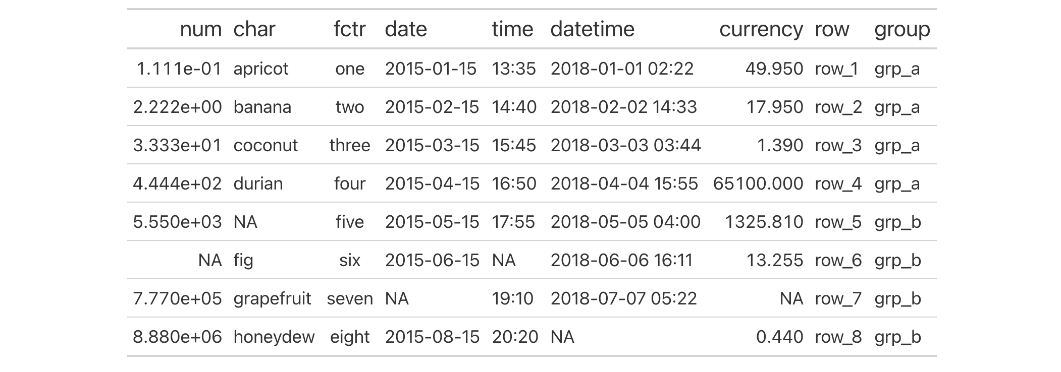
Function ID
8-3
Function Introduced
v0.2.0.5 (March 31, 2020)
See Also
Other helper functions:
adjust_luminance(),
cell_borders(),
cell_fill(),
cell_text(),
currency(),
default_fonts(),
escape_latex(),
from_column(),
google_font(),
gt_latex_dependencies(),
html(),
latex(),
md(),
nanoplot_options(),
pct(),
random_id(),
row_group(),
stub(),
system_fonts(),
unit_conversion()
Helper for creating a random id for a gt table
Description
random_id() can be used to create a random, character-based ID value
argument of variable length (the default is 10 letters).
Usage
random_id(n = 10)random_id(n = 10)
Arguments
n |
Number of letters
The |
Value
A character vector containing a single, random ID.
Function ID
8-28
Function Introduced
v0.2.0.5 (March 31, 2020)
See Also
Other helper functions:
adjust_luminance(),
cell_borders(),
cell_fill(),
cell_text(),
currency(),
default_fonts(),
escape_latex(),
from_column(),
google_font(),
gt_latex_dependencies(),
html(),
latex(),
md(),
nanoplot_options(),
pct(),
px(),
row_group(),
stub(),
system_fonts(),
unit_conversion()
Reaction rates for gas-phase atmospheric reactions of organic compounds
Description
The reactions dataset contains kinetic data for second-order (two body)
gas-phase chemical reactions for 1,683 organic compounds. The reaction-rate
values and parameters within this dataset are useful for studies of the
atmospheric environment. Organic pollutants, which are present in trace
amounts in the atmosphere, have been extensively studied by research groups
since their persistence in the atmosphere requires specific attention. Many
researchers have reported kinetic data on specific gas-phase reactions and
these mainly involve oxidation reactions with OH, nitrate radicals, ozone,
and chlorine atoms.
This compilation of rate constant (k) data as contains the values for rate
constants at 298 K (in units of cm^3 molecules^-1 s^-1) as well as
parameters that allow for the calculation of rate constants at different
temperatures (the temperature dependence parameters: A, B, and n).
Uncertainty values/factors and temperature limits are also provided here
where information is available.
Usage
reactionsreactions
Format
A tibble with 1,683 rows and 39 variables:
- compd_name
-
The name of the primary compound undergoing reaction with OH, ozone, NO3, or Cl.
- cmpd_mwt
-
The molecular weight of the compound in units of g/mol.
- cmpd_formula
-
The chemical formula of the compound.
- cmpd_type
-
The category of compounds that the
compd_namefalls under. - cmpd_smiles
-
The SMILES (simplified molecular-input line-entry system) representation for the compound.
- cmpd_inchi
-
The InChI (International Chemical Identifier) representation for the compound.
- cmpd_inchikey
-
The InChIKey, which is a hashed InChI value, has a fixed length of 27 characters. These values can be used to more easily perform database searches of chemical compounds.
- OH_k298
-
Rate constant at 298 K for OH reactions.
- OH_uncert
-
Uncertainty as a percentage for certain OH reactions.
- OH_u_fac
-
Uncertainty as a plus/minus difference for certain OH reactions.
- OH_a, OH_b, OH_n
-
Extended temperature dependence parameters for bimolecular OH reactions, to be used in the Arrhenius expression:
k(T)=A exp(-B/T) (T/300)^n. In that,Ais expressed as cm^3 molecules^-1 s^-1,Bis in units of K, andnis dimensionless. AnyNAvalues indicate that data is not available. - OH_t_low, OH_t_high
-
The low and high temperature boundaries (in units of K) for which the
OH_a,OH_b, andOH_nparameters are valid. - O3_k298
-
Rate constant at 298 K for ozone reactions.
- O3_uncert
-
Uncertainty as a percentage for certain ozone reactions.
- O3_u_fac
-
Uncertainty as a plus/minus difference for certain ozone reactions.
- O3_a, O3_b, O3_n
-
Extended temperature dependence parameters for bimolecular ozone reactions, to be used in the Arrhenius expression:
k(T)=A exp(-B/T) (T/300)^n. In that,Ais expressed as cm^3 molecules^-1 s^-1,Bis in units of K, andnis dimensionless. AnyNAvalues indicate that data is not available. - O3_t_low, O3_t_high
-
The low and high temperature boundaries (in units of K) for which the
O3_a,O3_b, andO3_nparameters are valid. - NO3_k298
-
Rate constant at 298 K for NO3 reactions.
- NO3_uncert
-
Uncertainty as a percentage for certain NO3 reactions.
- NO3_u_fac
-
Uncertainty as a plus/minus difference for certain NO3 reactions.
- NO3_a, NO3_b, NO3_n
-
Extended temperature dependence parameters for bimolecular NO3 reactions, to be used in the Arrhenius expression:
k(T)=A exp(-B/T) (T/300)^n. In that,Ais expressed as cm^3 molecules^-1 s^-1,Bis in units of K, andnis dimensionless. AnyNAvalues indicate that data is not available. - NO3_t_low, NO3_t_high
-
The low and high temperature boundaries (in units of K) for which the
NO3_a,NO3_b, andNO3_nparameters are valid. - Cl_k298
-
Rate constant at 298 K for Cl reactions.
- Cl_uncert
-
Uncertainty as a percentage for certain Cl reactions.
- Cl_u_fac
-
Uncertainty as a plus/minus difference for certain Cl reactions.
- Cl_a, Cl_b, Cl_n
-
Extended temperature dependence parameters for bimolecular Cl reactions, to be used in the Arrhenius expression:
k(T)=A exp(-B/T) (T/300)^n. In that,Ais expressed as cm^3 molecules^-1 s^-1,Bis in units of K, andnis dimensionless. AnyNAvalues indicate that data is not available. - Cl_t_low, Cl_t_high
-
The low and high temperature boundaries (in units of K) for which the
Cl_a,Cl_b, andCl_nparameters are valid.
Dataset ID and Badge
DATA-14

Dataset Introduced
v0.11.0 (July 9, 2024)
See Also
Other datasets:
constants,
countrypops,
exibble,
films,
gibraltar,
gtcars,
illness,
metro,
nuclides,
peeps,
photolysis,
pizzaplace,
rx_addv,
rx_adsl,
sp500,
sza,
towny
Examples
dplyr::glimpse(reactions)dplyr::glimpse(reactions)
A gt display table render function for use in Shiny
Description
With render_gt() we can create a reactive gt table that works
wonderfully once assigned to an output slot (with gt_output()). This
function is to be used within Shiny's server()
component. We have some options for controlling the size of the container
holding the gt table. The width and height arguments allow for sizing
the container, and the align argument allows us to align the table within
the container (some other fine-grained options for positioning are available
in tab_options()). If the table is interactive, the selected row indices
(relative to the underlying data, regardless of sorting) are available as
input$id, where id is the outputId used for this table in gt_output().
If the user has deselected all rows, the value is 0 (vs NULL when the
table initializes).
Usage
render_gt( expr, width = NULL, height = NULL, align = NULL, env = parent.frame(), quoted = FALSE, outputArgs = list() )render_gt( expr, width = NULL, height = NULL, align = NULL, env = parent.frame(), quoted = FALSE, outputArgs = list() )
Arguments
expr |
Expression
An expression that creates a gt table object. For sake of convenience,
a data frame or tibble can be used here (it will be automatically
introduced to |
width, height
|
Dimensions of table container
The width and height of the table's container. Either can be specified as a
single-length character vector with units of pixels or as a percentage. If
provided as a single-length numeric vector, it is assumed that the value is
given in units of pixels. The |
align |
Table alignment
The alignment of the table in its container. If |
env |
Evaluation environment
The environment in which to evaluate the |
quoted |
Option to
Is |
outputArgs |
Output arguments
A list of arguments to be passed through to the implicit call to
|
Value
An object of class shiny.render.function.
Examples
Here is a Shiny app (contained within a single file) that (1) prepares a
gt table, (2) sets up the ui with gt_output(), and (3) sets up the
server with a render_gt() that uses the gt_tbl object as the input
expression.
library(shiny)
gt_tbl <-
gtcars |>
gt() |>
fmt_currency(columns = msrp, decimals = 0) |>
cols_hide(columns = -c(mfr, model, year, mpg_c, msrp)) |>
cols_label_with(columns = everything(), fn = toupper) |>
data_color(columns = msrp, method = "numeric", palette = "viridis") |>
sub_missing() |>
opt_interactive(use_compact_mode = TRUE)
ui <- fluidPage(
gt_output(outputId = "table")
)
server <- function(input, output, session) {
output$table <- render_gt(expr = gt_tbl)
}
shinyApp(ui = ui, server = server)
Function ID
12-1
Function Introduced
v0.2.0.5 (March 31, 2020)
See Also
Other Shiny functions:
gt_output(),
gt_update_select()
Remove the table caption
Description
We can easily remove the caption text from a gt table with
rm_caption(). The caption may exist if it were set through the gt()
caption argument or via tab_caption().
This function for removal is useful if you have received a gt table
(perhaps through an API that returns gt objects) but would prefer that
the table not have a caption at all. This function is safe to use even if
there is no table caption set in the input gt_tbl object.
Usage
rm_caption(data)rm_caption(data)
Arguments
data |
The gt table data object
This is the gt table object that is commonly created through use of the
|
Value
An object of class gt_tbl.
Examples
Use a portion of the gtcars dataset to create a gt table. We'll add a
header part with tab_header(), and, a caption will also be added via
tab_caption().
gt_tbl <-
gtcars |>
dplyr::select(mfr, model, msrp) |>
dplyr::slice(1:5) |>
gt() |>
tab_header(
title = md("Data listing from **gtcars**"),
subtitle = md("`gtcars` is an R dataset")
) |>
tab_caption(caption = md("**gt** table example."))
gt_tbl

If you decide that you don't want the caption in the gt_tbl object, it can
be removed with rm_caption().
rm_caption(data = gt_tbl)

Function ID
7-6
Function Introduced
v0.8.0 (November 16, 2022)
See Also
Other part removal functions:
rm_footnotes(),
rm_header(),
rm_source_notes(),
rm_spanners(),
rm_stubhead()
Remove table footnotes
Description
If you have one or more footnotes that ought to be removed, rm_footnotes()
allows for such a selective removal. The table footer is an optional table
part that is positioned below the table body, containing areas for both the
footnotes and source notes.
This function for removal is useful if you have received a gt table
(perhaps through an API that returns gt objects) but would prefer that
some or all of the footnotes be removed. This function is safe to use even if
there are no footnotes in the input gt_tbl object so long as select helpers
(such as the default everything()) are used instead of explicit integer
values.
Usage
rm_footnotes(data, footnotes = everything())rm_footnotes(data, footnotes = everything())
Arguments
data |
The gt table data object
This is the gt table object that is commonly created through use of the
|
footnotes |
Footnotes to remove
A specification of which footnotes should be removed. The footnotes to be
removed can be given as a vector of integer values (they are stored as
integer positions, in order of creation, starting at |
Value
An object of class gt_tbl.
Examples
Use a subset of the sza dataset to create a gt table. Color the sza
column using data_color(), then, use tab_footnote() twice to
add two footnotes (each one targeting a different column label).
gt_tbl <-
sza |>
dplyr::filter(
latitude == 20 &
month == "jan" &
!is.na(sza)
) |>
dplyr::select(-latitude, -month) |>
gt() |>
data_color(
columns = sza,
palette = c("white", "yellow", "navyblue"),
domain = c(0, 90)
) |>
tab_footnote(
footnote = "Color indicates height of sun.",
locations = cells_column_labels(
columns = sza
)
) |>
tab_footnote(
footnote = "
The true solar time at the given latitude
and date (first of month) for which the
solar zenith angle is calculated.
",
locations = cells_column_labels(
columns = tst
)
) |>
cols_width(everything() ~ px(150))
gt_tbl
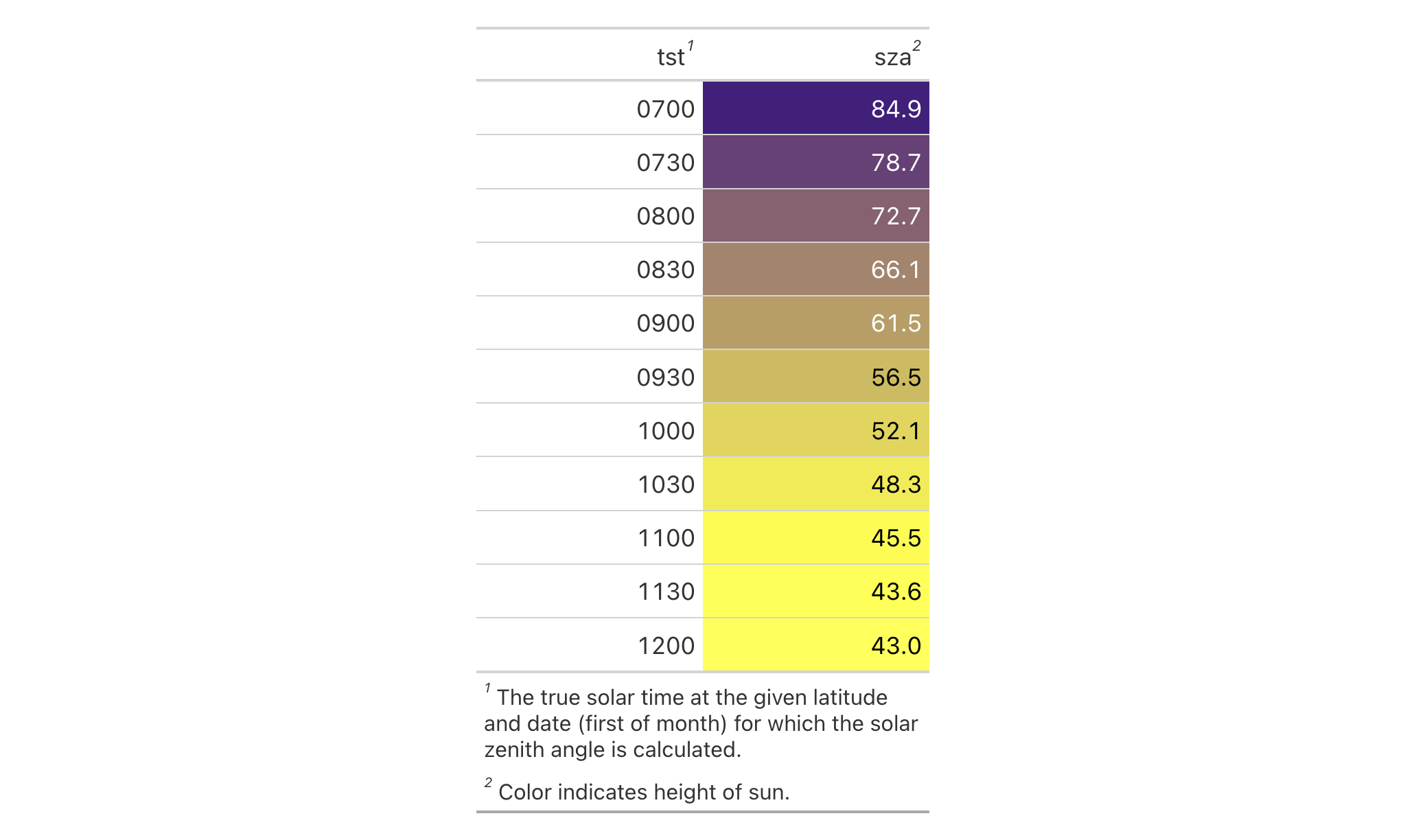
If you decide that you don't want the footnotes in the gt_tbl object,
they can be removed with rm_footnotes().
rm_footnotes(data = gt_tbl)
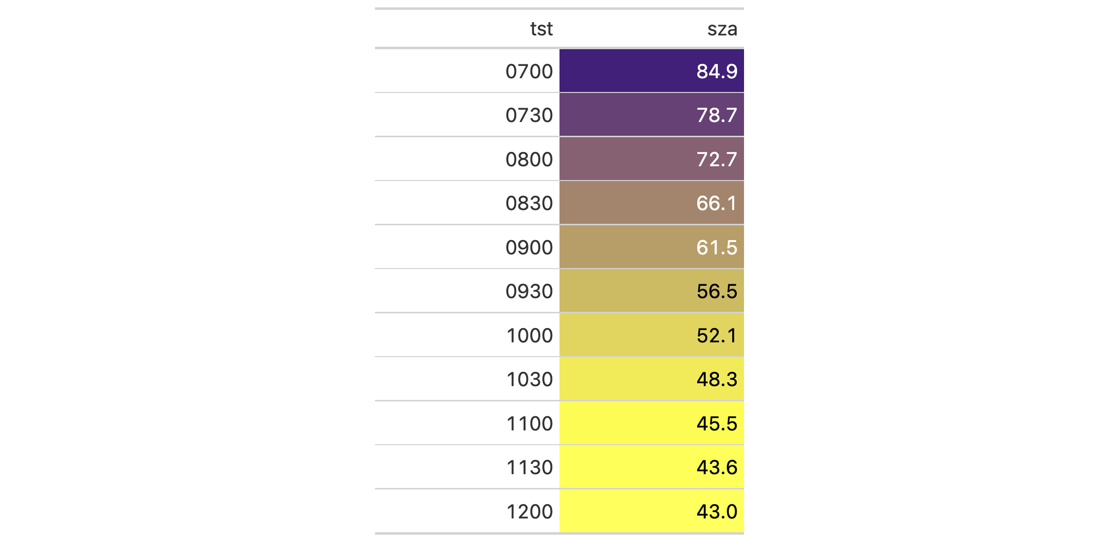
Individual footnotes can be selectively removed. Footnotes are identified by
their index values. To remove the footnote concerning true solar time
(footnote 2, since it was supplied to gt after the other footnote) we
would give the correct index value to footnotes.
rm_footnotes(data = gt_tbl, footnotes = 2)

Function ID
7-4
Function Introduced
v0.8.0 (November 16, 2022)
See Also
Other part removal functions:
rm_caption(),
rm_header(),
rm_source_notes(),
rm_spanners(),
rm_stubhead()
Remove the table header
Description
We can remove the table header from a gt table quite easily with
rm_header(). The table header is an optional table part (positioned above
the column labels) that can be added through tab_header().
This function for removal is useful if you have received a gt table
(perhaps through an API that returns gt objects) but would prefer that
the table not contain a header. This function is safe to use even if there is
no header part in the input gt_tbl object.
Usage
rm_header(data)rm_header(data)
Arguments
data |
The gt table data object
This is the gt table object that is commonly created through use of the
|
Value
An object of class gt_tbl.
Examples
Let's use a subset of the gtcars dataset to create a gt table. A
header part can be added with tab_header(); with that, we get
a title and a subtitle for the table.
gt_tbl <-
gtcars |>
dplyr::select(mfr, model, msrp) |>
dplyr::slice(1:5) |>
gt() |>
tab_header(
title = md("Data listing from **gtcars**"),
subtitle = md("`gtcars` is an R dataset")
)
gt_tbl

If you decide that you don't want the header in the gt_tbl object, it can
be removed with rm_header().
rm_header(data = gt_tbl)

Function ID
7-1
Function Introduced
v0.8.0 (November 16, 2022)
See Also
Other part removal functions:
rm_caption(),
rm_footnotes(),
rm_source_notes(),
rm_spanners(),
rm_stubhead()
Remove table source notes
Description
If you have one or more source notes that ought to be removed,
rm_source_notes() allows for such a selective removal. The table footer is
an optional table part that is positioned below the table body, containing
areas for both the source notes and footnotes.
This function for removal is useful if you have received a gt table
(perhaps through an API that returns gt objects) but would prefer that
some or all of the source notes be removed. This function is safe to use even
if there are no source notes in the input gt_tbl object so long as select
helpers (such as the default everything()) are used instead of explicit
integer values.
Usage
rm_source_notes(data, source_notes = everything())rm_source_notes(data, source_notes = everything())
Arguments
data |
The gt table data object
This is the gt table object that is commonly created through use of the
|
source_notes |
Source notes to remove
A specification of which source notes should be removed. The source notes
to be removed can be given as a vector of integer values (they are stored
as integer positions, in order of creation, starting at |
Value
An object of class gt_tbl.
Examples
Use a subset of the gtcars dataset to create a gt table.
tab_source_note() is used to add a source note to the table footer that
cites the data source (or, it could just be arbitrary text). We'll use the
function twice, in effect adding two source notes to the footer.
gt_tbl <- gtcars |> dplyr::select(mfr, model, msrp) |> dplyr::slice(1:5) |> gt() |> tab_source_note(source_note = "Data from the 'edmunds.com' site.") |> tab_source_note(source_note = "Showing only the first five rows.") |> cols_width(everything() ~ px(120)) gt_tbl

If you decide that you don't want the source notes in the gt_tbl object,
they can be removed with rm_source_notes().
rm_source_notes(data = gt_tbl)

Individual source notes can be selectively removed. Source notes are
identified by their index values. To remove the source note concerning the
extent of the data (source note 2, since it was supplied to gt after
the other source note) we would give the correct index value to
source_notes.
rm_source_notes(data = gt_tbl, source_notes = 2)

Function ID
7-5
Function Introduced
v0.8.0 (November 16, 2022)
See Also
Other part removal functions:
rm_caption(),
rm_footnotes(),
rm_header(),
rm_spanners(),
rm_stubhead()
Remove column spanner labels
Description
If you would like to remove column spanner labels then the rm_spanners()
function can make this possible. Column spanner labels appear above the
column labels and can occupy several levels via stacking either through
tab_spanner() or tab_spanner_delim(). Spanner column labels are
distinguishable and accessible by their ID values.
This function for removal is useful if you have received a gt table
(perhaps through an API that returns gt objects) but would prefer that
some or all of the column spanner labels be removed. This function is safe to
use even if there are no column spanner labels in the input gt_tbl object
so long as select helpers (such as the default everything()) are used
instead of explicit ID values.
Usage
rm_spanners(data, spanners = everything(), levels = NULL)rm_spanners(data, spanners = everything(), levels = NULL)
Arguments
data |
The gt table data object
This is the gt table object that is commonly created through use of the
|
spanners |
Spanners to remove
A specification of which spanner column labels should be removed. Those to
be removed can be given as a vector of spanner ID values (every spanner
column label has one, either set by the user or by gt when using
|
levels |
Spanner levels to remove
Instead of removing spanner column labels by ID values, entire levels of
spanners can instead be removed. Supply a numeric vector of level values
(the first level is |
Value
An object of class gt_tbl.
Examples
Use a portion of the gtcars dataset to create a gt table. With
tab_spanner(), we can group several related columns together under a
spanner column. In this example, that is done with several tab_spanner()
calls in order to create two levels of spanner column labels.
gt_tbl <-
gtcars |>
dplyr::select(
-mfr, -trim, bdy_style, drivetrain,
-drivetrain, -trsmn, -ctry_origin
) |>
dplyr::slice(1:8) |>
gt(rowname_col = "model") |>
tab_spanner(label = "HP", columns = c(hp, hp_rpm)) |>
tab_spanner(label = "Torque", columns = c(trq, trq_rpm)) |>
tab_spanner(label = "MPG", columns = c(mpg_c, mpg_h)) |>
tab_spanner(
label = "Performance",
columns = c(
hp, hp_rpm, trq, trq_rpm,
mpg_c, mpg_h
)
)
gt_tbl
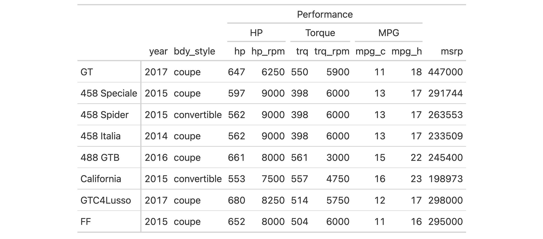
If you decide that you don't want any of the spanners in the gt_tbl object,
they can all be removed with rm_spanners().
rm_spanners(data = gt_tbl)
Individual spanner column labels can be removed by ID value. In all the above
uses of tab_spanner(), the label value is the ID value (you can
alternately set a different ID value though the id argument). Let's remove
the "HP" and "MPG" spanner column labels with rm_spanners().
rm_spanners(data = gt_tbl, spanners = c("HP", "MPG"))
We can also remove spanner column labels by level with rm_spanners().
Provide a vector of one or more values greater than or equal to 1 (the
first level starts there). In the next example, we'll remove the first level
of spanner column labels. Any levels not being removed will collapse down
accordingly.
rm_spanners(data = gt_tbl, levels = 1)
Function ID
7-3
Function Introduced
v0.8.0 (November 16, 2022)
See Also
Other part removal functions:
rm_caption(),
rm_footnotes(),
rm_header(),
rm_source_notes(),
rm_stubhead()
Remove the stubhead label
Description
We can easily remove the stubhead label from a gt table with
rm_stubhead(). The stubhead location only exists if there is a table stub
and the text in that cell is added with tab_stubhead().
This function for removal is useful if you have received a gt table
(perhaps through an API that returns gt objects) but would prefer that
the table not contain any content in the stubhead. This function is safe to
use even if there is no stubhead label in the input gt_tbl object.
Usage
rm_stubhead(data)rm_stubhead(data)
Arguments
data |
The gt table data object
This is the gt table object that is commonly created through use of the
|
Value
An object of class gt_tbl.
Examples
Using the gtcars dataset, we'll create a gt table. With
tab_stubhead(), it's possible to add a stubhead label. This appears in the
top-left and can be used to describe what is in the stub.
gt_tbl <- gtcars |> dplyr::select(model, year, hp, trq) |> dplyr::slice(1:5) |> gt(rowname_col = "model") |> tab_stubhead(label = "car") gt_tbl

If you decide that you don't want the stubhead label in the gt_tbl object,
it can be removed with rm_stubhead().
rm_stubhead(data = gt_tbl)

Function ID
7-2
Function Introduced
v0.8.0 (November 16, 2022)
See Also
Other part removal functions:
rm_caption(),
rm_footnotes(),
rm_header(),
rm_source_notes(),
rm_spanners()
Select helper for targeting the row group column
Description
Should you need to target only the row group column for column-width
declarations (i.e., when row_group_as_column = TRUE is set in the initial
gt() call), the row_group() select helper can be used. This shorthand
makes it so you don't have to use the name of the column that was selected
as the row group column.
Usage
row_group()row_group()
Value
A character vector of class "row_group_column".
Examples
Create a tibble that has a row column (values from 1 to 6), a group
column, and a vals column (containing the same values as in row).
tbl <-
dplyr::tibble(
row = 1:6,
group = c(rep("Group A", 3), rep("Group B", 3)),
vals = 1:6
)
Create a gt table with a two-column stub (incorporating the row and
group columns in that). We can set the widths of the two columns in the
stub with the row_group() and stub() helpers on the LHS of the
expressions passed to cols_width().
tbl |>
gt(
rowname_col = "row",
groupname_col = "group",
row_group_as_column = TRUE
) |>
fmt_roman(columns = stub()) |>
cols_width(
row_group() ~ px(200),
stub() ~ px(100),
vals ~ px(50)
)

Function ID
8-11
Function Introduced
v0.11.0 (July 9, 2024)
See Also
Other helper functions:
adjust_luminance(),
cell_borders(),
cell_fill(),
cell_text(),
currency(),
default_fonts(),
escape_latex(),
from_column(),
google_font(),
gt_latex_dependencies(),
html(),
latex(),
md(),
nanoplot_options(),
pct(),
px(),
random_id(),
stub(),
system_fonts(),
unit_conversion()
Modify the ordering of any row groups
Description
We can modify the display order of any row groups in a gt object with
row_group_order(). The groups argument takes a vector of row group ID
values. After this function is invoked, the row groups will adhere to this
revised ordering. It isn't necessary to provide all row ID values in
groups, rather, what is provided will assume the specified ordering at the
top of the table and the remaining row groups will follow in their original
ordering.
Usage
row_group_order(data, groups)row_group_order(data, groups)
Arguments
data |
The gt table data object
This is the gt table object that is commonly created through use of the
|
groups |
Specification of row group IDs
A character vector of row group ID values corresponding to the revised ordering. While this vector must contain valid group ID values, it is not required to have all of the row group IDs within it; any omitted values will be added to the end while preserving the original ordering. |
Value
An object of class gt_tbl.
Examples
Let's use exibble to create a gt table with a stub and with row
groups. We can modify the order of the row groups with row_group_order(),
specifying the new ordering in groups.
exibble |>
dplyr::select(char, currency, row, group) |>
gt(
rowname_col = "row",
groupname_col = "group"
) |>
row_group_order(groups = c("grp_b", "grp_a"))
Function ID
6-3
Function Introduced
v0.2.0.5 (March 31, 2020)
See Also
Other row addition/modification functions:
grand_summary_rows(),
row_order(),
rows_add(),
rows_hide(),
rows_unhide(),
summary_columns(),
summary_rows()
Modify the order of rows within groups
Description
We can modify the display order of rows within any row groups in a gt
object with row_order(). One or more column names can be provided to define
the sorting criteria. By default, rows are sorted in ascending order; use
reverse = TRUE to sort in descending order. The ordering is applied lazily
during the table build phase, ensuring it works alongside other row-reordering
operations.
Usage
row_order(data, ..., groups = NULL, reverse = FALSE)row_order(data, ..., groups = NULL, reverse = FALSE)
Arguments
data |
The gt table data object
This is the gt table object that is commonly created through use of the
|
... |
Column expressions for ordering
Column names or expressions describing how to order the rows. Multiple columns can be specified for hierarchical sorting, where the first column is the primary sort key. |
groups |
Specification of row group IDs
An optional character vector of row group ID values to target. If |
reverse |
Reverse the sort order
Should the sort order be reversed (i.e., descending)? By default this is
|
Value
An object of class gt_tbl.
Examples
Let's use the gtcars dataset to demonstrate row ordering within groups.
We'll create a gt table grouped by country and then order rows within
each group by the car price in descending order.
gtcars |>
dplyr::select(mfr, model, ctry_origin, msrp) |>
dplyr::filter(ctry_origin %in% c("Japan", "United Kingdom")) |>
dplyr::slice_head(n = 12) |>
gt(groupname_col = "ctry_origin") |>
row_order(msrp, reverse = TRUE) |>
fmt_currency(columns = msrp, decimals = 0) |>
tab_options(column_labels.hidden = TRUE)
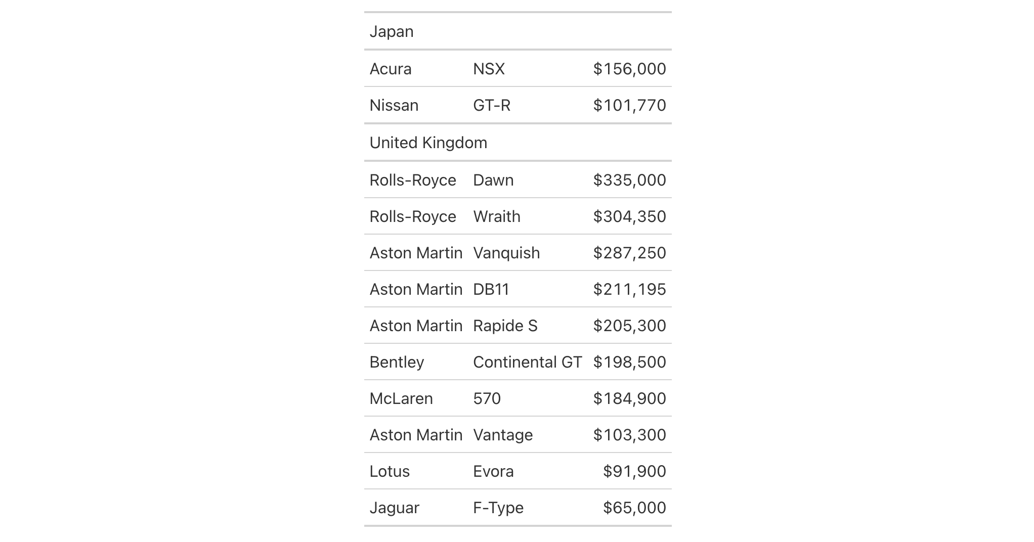
Using towny, we can order rows only within specific groups. Here we
order Ontario municipalities by population density in 2021, but only for
the "city" and "town" groups (leaving "township" rows in their original
order):
towny |>
dplyr::filter(csd_type %in% c("city", "town", "township")) |>
dplyr::select(name, csd_type, population_2021, density_2021) |>
dplyr::slice_head(n = 5, by = csd_type) |>
gt(groupname_col = "csd_type") |>
fmt_integer(columns = population_2021) |>
fmt_number(columns = density_2021, decimals = 1) |>
row_order(density_2021, groups = c("city", "town"), reverse = TRUE)
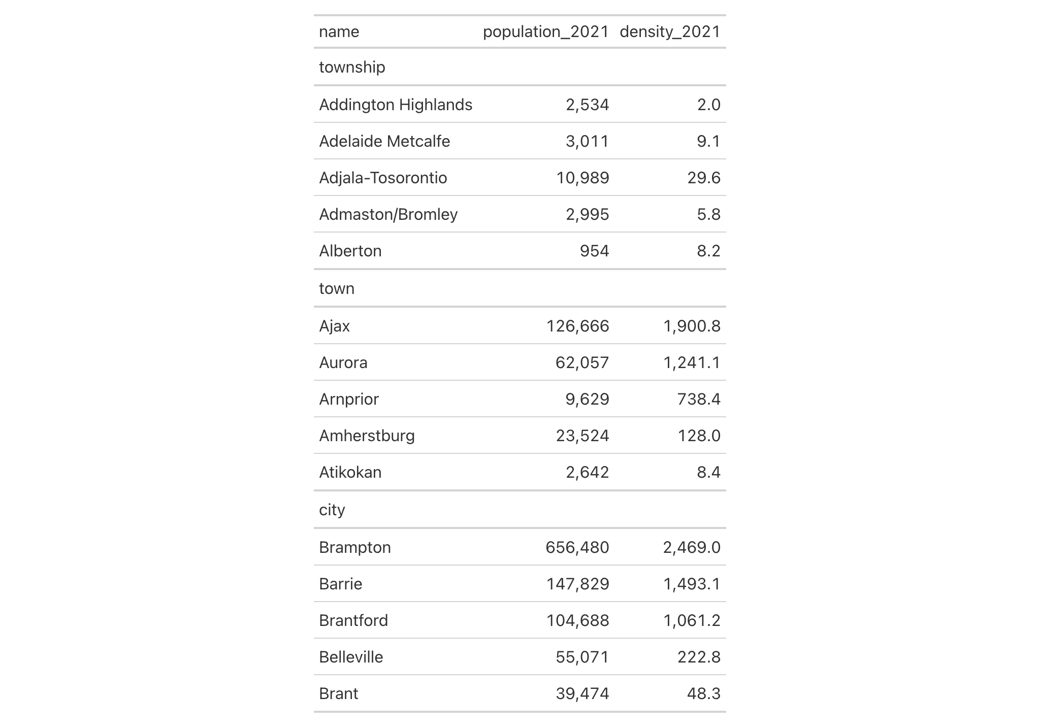
Using countrypops, multiple sorting columns can be specified for
hierarchical ordering. Here we create a table grouped by year, and sort
countries by population within each year:
countrypops |>
filter(country_code_2 %in% c("BR", "RU", "IN", "CN", "US", "ID")) |>
filter(year %in% c(2000, 2010, 2020)) |>
select(year, country_name, population) |>
gt(groupname_col = "year", row_group_as_column = TRUE) |>
fmt_integer(columns = population) |>
row_order(population, reverse = TRUE) |>
opt_vertical_padding(scale = 0.5)
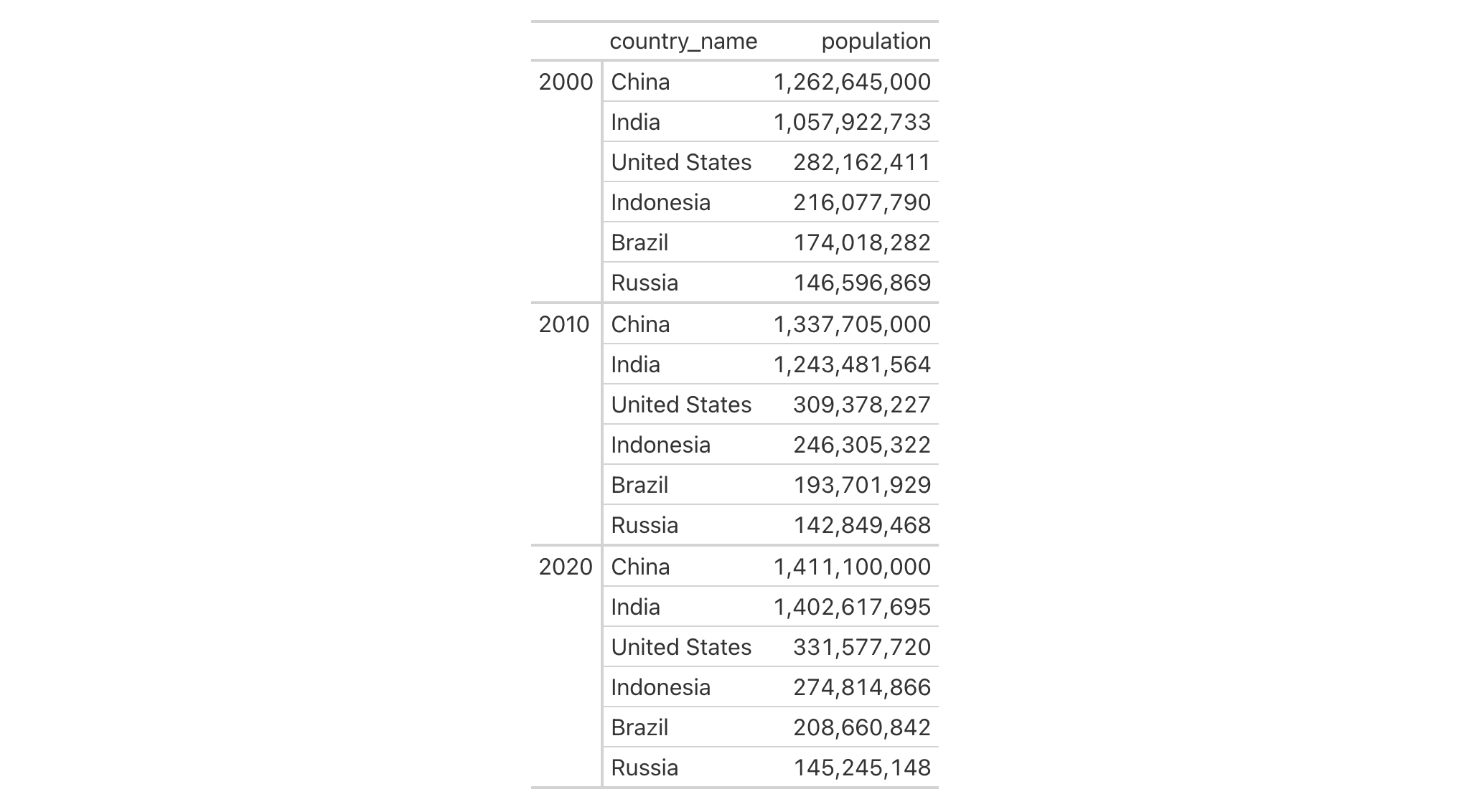
Function ID
6-4
Function Introduced
v1.3.0 (January 22, 2026)
See Also
row_group_order(), which orders the groups themselves.
Other row addition/modification functions:
grand_summary_rows(),
row_group_order(),
rows_add(),
rows_hide(),
rows_unhide(),
summary_columns(),
summary_rows()
Add one or more rows to a gt table
Description
It's possible to add new rows to your table with rows_add() by supplying
the new row data through name-value pairs or two-sided formula expressions.
The new rows are added to the bottom of the table by default but can be added
internally by using either the .before or .after arguments. If entirely
empty rows need to be added, the .n_empty option provides a means to
specify the number of blank (i.e., all NA) rows to be inserted into the
table.
Usage
rows_add( .data, ..., .list = list2(...), .before = NULL, .after = NULL, .n_empty = NULL )rows_add( .data, ..., .list = list2(...), .before = NULL, .after = NULL, .n_empty = NULL )
Arguments
.data |
The gt table data object
This is the gt table object that is commonly created through use of the
|
... |
Cell data assignments
Expressions for the assignment of cell values to the new rows by column
name in |
.list |
Alternative to
Allows for the use of a list as an input alternative to |
.before, .after
|
Row used as anchor
A single row-resolving expression or row index an be given to either
|
.n_empty |
Number of empty rows to add
An option to add empty rows in lieu of rows containing data that would
otherwise be supplied to |
Value
An object of class gt_tbl.
Targeting the row for insertion with .before or .after
The targeting of a row for insertion is done through the .before or
.after arguments (only one of these options should be used). This can be
done in a variety of ways. If a stub is present, then we potentially have row
identifiers. This is the ideal method to use for establishing a row target.
We can use tidyselect-style expressions to target a row. It's also
possible to use row indices (e.g., c(3, 5, 6)) though these index values
must correspond to the row numbers of the input data (the indices won't
necessarily match those of rearranged rows if row groups are present). One
more type of expression is possible, an expression that takes column values
(can involve any of the available columns in the table) and returns a logical
vector.
Examples
Let's make a simple gt table with the exibble dataset, using the
row column for labels in the stub. We'll add a single row to the bottom of
the table with rows_add(). With name-value pairs, it's possible to add
values for the new body cells that correspond to columns available in the
table. For any columns that are missed, the related body cells will receive
NA values.
exibble |>
gt(rowname_col = "row") |>
rows_add(
row = "row_9",
num = 9.999E7,
char = "ilama",
fctr = "nine",
group = "grp_b"
)

If you wanted to place a row somewhere in the middle of the table, we can use
either of the .before or .after arguments in rows_add():
exibble |>
gt(rowname_col = "row") |>
rows_add(
row = "row_4.5",
num = 9.923E3,
char = "elderberry",
fctr = "eighty",
group = "grp_a",
.after = "row_4"
)

Putting a row at the beginning requires the use of the .before argument. We
can use an index value for the row as in .before = 1 for maximum easiness:
exibble |>
gt(rowname_col = "row") |>
rows_add(
row = "row_0",
num = 0,
char = "apple",
fctr = "zero",
group = "grp_a",
.before = 1
)

Again with exibble, we can create an example where we insert 'spacer'
rows. These are rows without any content and merely serve to add extra
vertical space to the table in specific locations. In this case, we'll have a
stub with row names and row groups (set up in the gt() call). The two rows
being added will occupy the bottom row of each group. The only data defined
for the two rows involves values for the row and group columns. It's
important that the data for group uses the group names already present in
the data ("grp_a" and "grp_b"). The corresponding values for row will
be "row_a_end" and "row_b_end", these will be used later expressions for
targeting the rows. Here's the code needed to generate spacer rows at the end
of each row group:
exibble |>
gt(rowname_col = "row", groupname_col = "group") |>
rows_add(
row = c("row_a_end", "row_b_end"),
group = c("grp_a", "grp_b")
) |>
tab_style(
style = cell_borders(sides = "top", style = "hidden"),
locations = list(
cells_body(rows = ends_with("end")),
cells_stub(rows = ends_with("end"))
)
) |>
sub_missing(missing_text = "") |>
text_case_when(
grepl("end", x) ~ "",
.locations = cells_stub()
) |>
opt_vertical_padding(scale = 0.5)

All missing values were substituted with an empty string (""), and that was
done by using sub_missing(). We removed the top border of the
new rows with a call to tab_style(), targeting those rows where the row
labels end with "end". Finally, we get rid of the row labels with the use
of text_case_when(), using a similar strategy of targeting the
name of the row label.
Another application is starting from nothing (really just the definition of
columns) and building up a table using several invocations of rows_add().
This might be useful in interactive or programmatic applications. Here's an
example where two columns are defined with dplyr::tibble()
(and no rows are present initially); with two calls of rows_add(), two
separate rows are added.
dplyr::tibble(
time = lubridate::POSIXct(),
event = character(0L)
) |>
gt() |>
rows_add(
time = lubridate::ymd_hms("2022-01-23 12:36:10"),
event = "start"
) |>
rows_add(
time = lubridate::ymd_hms("2022-01-23 13:41:26"),
event = "completed"
)

It's possible to use formula syntax in rows_add() to perform column
resolution along with attaching values for new rows. If we wanted to use an
equivalent value for multiple cells in a new row, a valid input would be in
the form of <expr> ~ <value vector>. In the following example, we create a
simple table with six columns (the rendered gt table displays four
columns and a stub column since the group column is used for row group
labels). Let's add a single row where some of the cell values added
correspond to columns are resolved on the LHS of the formula expressions:
dplyr::tibble(
group = c("Group A", "Group B", "Group B"),
id = c("WG-025360", "WG-025361", "WG-025362"),
a = c(1, 6, 2),
b = c(2, 6, 2),
quantity_x = c(83.58, 282.71, 92.20),
quantity_y = c(36.82, 282.71, 87.34)
) |>
gt(rowname_col = "id", groupname_col = "group") |>
rows_add(
starts_with("gr") ~ "Group A",
id = "WG-025363",
c(a, b) ~ 5,
starts_with("quantity") ~ 72.63
)

We can see that using starts_with("gr") yields a successful match to the
group column with the tangible result being an addition of a row to the
"Group A" group (the added row is the second one in the rendered gt
table). Through the use of c(a, b), it was possible to add the value 5 to
both the a and b columns. A similar approach was taken with adding the
72.63 value to the quantity_x and quantity_y columns though we used the
starts_with("quantity") expression to get gt to resolve those two
columns.
You can start with an empty table (i.e., no columns and no rows) and add one
or more rows to it. In the completely empty table scenario, where you would
use something like dplyr::tibble() or data.frame() with gt(), the first
rows_add() could have rows of arbitrary width. In other words, you get to
generate table columns (and rows) with a completely empty table via
rows_add(). Here's an example of that:
gt(dplyr::tibble()) |>
rows_add(
msrp = c(29.95, 49.95, 79.95),
item = c("Klax", "Rez", "Ys"),
type = c("A", "B", "X")
) |>
rows_add(
msrp = 14.95,
item = "D",
type = "Z"
)

In the above, three columns and three rows were generated. The second usage
of rows_add() had to use of a subset of those columns (all three were used
to create a complete, new row).
We can also start with a virtually empty table: one that has columns but no
actual rows. With this type of multi-column, zero-row table, one needs to use
a subset of the columns when generating new rows through rows_add().
dplyr::tibble(
msrp = numeric(0L),
item = character(0L),
type = character(0L)
) |>
gt() |>
rows_add(
msrp = c(29.95, 49.95, 79.95, 14.95),
item = c("Klax", "Rez", "Ys", "D"),
type = c("A", "B", "X", "Z")
) |>
cols_add(
genre = c("puzzle", "action", "RPG", "adventure")
) |>
fmt_currency() |>
cols_move_to_end(columns = msrp)

Function ID
6-5
Function Introduced
v0.10.0 (October 7, 2023)
See Also
Other row addition/modification functions:
grand_summary_rows(),
row_group_order(),
row_order(),
rows_hide(),
rows_unhide(),
summary_columns(),
summary_rows()
Hide one or more rows
Description
rows_hide() allows us to hide one or more rows from appearing in the final
output table. While it's possible and often desirable to omit rows from the
input table data before introduction to gt(), there can be cases where the
data in certain rows is useful (as a row reference during formatting of other
rows or for column-based aggregations) but the final display of those rows is
not necessary.
Usage
rows_hide(data, rows)rows_hide(data, rows)
Arguments
data |
The gt table data object
This is the gt table object that is commonly created through use of the
|
rows |
Rows to target
The rows to hide in the output display table. Can either be a series of row
IDs provided in |
Details
The hiding of rows is internally a rendering directive, so, all rows that are
'hidden' are still accessible and useful in any expression provided to a
rows argument. Furthermore, rows_hide() (as with many gt functions)
can be placed anywhere in a pipeline of gt function calls (acting as a
promise to hide rows when the timing is right). However, there's perhaps
greater readability when placing this call closer to the end of such a
pipeline.
Note that when using summary_rows() or grand_summary_rows(), the
aggregation calculations will only include the visible rows. Hidden rows are
excluded from summary computations. This allows summary values to dynamically
reflect the currently visible data.
rows_hide() quietly changes the visible state of a row (much like
rows_unhide()) and doesn't yield warnings or messages when changing the
state of already-hidden rows.
Value
An object of class gt_tbl.
Examples
Let's use a small portion of the countrypops dataset to create a gt
table. We can hide rows where the population is below a certain threshold
using rows_hide().
countrypops |>
dplyr::filter(
country_name == "Egypt",
year %in% 2017:2021
) |>
gt(rowname_col = "year") |>
fmt_integer(columns = population) |>
rows_hide(rows = population < 100E6)

Using another countrypops-based gt table, we can hide specific rows
by targeting them with their row labels (from the stub). Note that the
footnote placement still works correctly, skipping the hidden rows in its
mark indexing.
countrypops |>
dplyr::filter(
country_name == "Brazil",
year %in% 2017:2021
) |>
gt(rowname_col = "year") |>
fmt_integer(columns = population) |>
rows_hide(rows = c("2018", "2020")) |>
tab_footnote(
footnote = "Population above 210,000,000.",
locations = cells_body(
columns = population,
rows = population > 210E6
)
)

Function ID
6-7
Function Introduced
In Development
See Also
Other row addition/modification functions:
grand_summary_rows(),
row_group_order(),
row_order(),
rows_add(),
rows_unhide(),
summary_columns(),
summary_rows()
Unhide one or more rows
Description
rows_unhide() allows us to take one or more hidden rows (usually done
via rows_hide()) and make them visible in the final output table. This may
be important in cases where the user obtains a gt_tbl object with hidden
rows and there is motivation to reveal one or more of those.
Usage
rows_unhide(data, rows)rows_unhide(data, rows)
Arguments
data |
The gt table data object
This is the gt table object that is commonly created through use of the
|
rows |
Rows to target
The rows to unhide in the output display table. Can either be a series of
row IDs provided in |
Details
The hiding and unhiding of rows is internally a rendering directive, so, all
rows that are 'hidden' are still accessible and useful in any expression
provided to a rows argument. The rows_unhide() function quietly changes
the visible state of a row (much like the rows_hide() function) and doesn
doesn't yield warnings or messages when changing the state of already-visible
rows.
Note that unhiding rows will cause them to be included in any summary_rows()
or grand_summary_rows() calculations, as these aggregations only operate on
visible rows.
Value
An object of class gt_tbl.
Examples
Let's use a small portion of the countrypops dataset to create a gt
table. We'll hide all rows but then unhide specific ones.
tab_1 <-
countrypops |>
dplyr::filter(
country_name == "Japan",
year %in% 2017:2021
) |>
gt(rowname_col = "year") |>
fmt_integer(columns = population) |>
rows_hide(rows = everything())
tab_1

If we obtain the tab_1 object without access to the code or source data,
and we want to reveal otherwise hidden rows, then rows_unhide() becomes
useful.
tab_1 |> rows_unhide(rows = c("2019", "2021"))

Function ID
6-8
Function Introduced
In Development
See Also
Other row addition/modification functions:
grand_summary_rows(),
row_group_order(),
row_order(),
rows_add(),
rows_hide(),
summary_columns(),
summary_rows()
Apply conditional formatting to cells with rows and columns
Description
To apply styling or formatting, you can use the
columns and rows arguments. The syntax should be very familiar for dplyr
users as you can use the tidyselect specification.
Targeting of values is done through columns and additionally by rows (if
nothing is provided for rows then entire columns are selected). The
columns argument allows us to target a subset of cells contained in the
resolved columns. We say resolved because aside from declaring column names
in c() (with bare column names or names in quotes) we can use
tidyselect-style expressions. This can be as basic as supplying a select
helper like starts_with(), or, providing a more complex incantation like
where(~ is.numeric(.x) & max(.x, na.rm = TRUE) > 1E6)
which targets numeric columns that have a maximum value greater than
1,000,000 (excluding any NAs from consideration).
By default all columns and rows are selected (with the everything()
defaults). Cell values that are incompatible with a given formatting function
will be skipped over, like character values and numeric fmt_*()
functions. So it's safe to select all columns with a particular formatting
function (only those values that can be formatted will be formatted), but,
you may not want that. One strategy is to format the bulk of cell values with
one formatting function and then constrain the columns for later passes with
other types of formatting (the last formatting done to a cell is what you get
in the final output).
Once the columns are targeted, we may also target the rows within those
columns. This can be done in a variety of ways. If a stub is present, then we
potentially have row identifiers. Those can be used much like column names in
the columns-targeting scenario. We can use simpler tidyselect-style
expressions (the select helpers should work well here) and we can use quoted
row identifiers in c(). It's also possible to use row indices (e.g.,
c(3, 5, 6)) though these index values must correspond to the row numbers of
the input data (the indices won't necessarily match those of rearranged rows
if row groups are present). One more type of expression is possible, an
expression that takes column values (can involve any of the available columns
in the table) and returns a logical vector. This is nice if you want to base
formatting on values in the column or another column, or, you'd like to use a
more complex predicate expression.
Examples
gt_tbl <- gt(exibble) gt_tbl |> fmt_time( columns = contains("time") & !starts_with("date"), rows = num > 100 & group == "grp_b" ) # Styling numeric columns based on range gt_tbl |> tab_style( style = cell_text(weight = "bold"), locations = cells_body(columns = where(is.factor)) ) # Naming rows gt_tbl_rows <- gt(exibble, rowname_col = "row") gt_tbl_rows |> fmt_datetime( columns = datetime, rows = c("row_1", "row_8") )gt_tbl <- gt(exibble) gt_tbl |> fmt_time( columns = contains("time") & !starts_with("date"), rows = num > 100 & group == "grp_b" ) # Styling numeric columns based on range gt_tbl |> tab_style( style = cell_text(weight = "bold"), locations = cells_body(columns = where(is.factor)) ) # Naming rows gt_tbl_rows <- gt(exibble, rowname_col = "row") gt_tbl_rows |> fmt_datetime( columns = datetime, rows = c("row_1", "row_8") )
An ADDV-flavored clinical trial toy dataset
Description
This tibble contains artificial protocol deviation data for 180 subjects
in the Intent-to-Treat (ITT) population of the GT01 study. The dataset
contains the usual parameters (PARAM, PARAMCD) for an addv. There is
summary parameter (PARCAT1 == "OVERALL") for each subject of the GT01
ITT-population, indicating whether or not at least one major protocol
deviation (PD) occurred throughout the course of the study for the respective
subject. Individual records for protocol deviations per subject exist,
indicating which specific type of PD occurred. The additional flag CRIT1FL,
shows whether a PD was related to COVID-19 or not.
Although the data was intentionally created to mimic a typical clinical trial dataset following the CDISC format, it might not strictly comply with CDISC ADaM rules. The intent is to showcase the workflow for clinical table creation rather than creating a fully CDISC-compliant ADaM dataset.
Usage
rx_addvrx_addv
Format
A tibble with 291 rows and 20 variables:
- STUDYID, STUDYIDN
-
The unique study identifier and its numeric version.
- USUBJID
-
The unique subject identifier.
- TRTA, TRTAN
-
The study intervention and its numeric version, which is either
"Placebo"(1),"Drug 1"(2), orNA(3), missing for screen failures). - ITTFL
-
Intent-to-Treat (ITT) population flag, where
"Y"indicates a subject belongs to the ITT population and"N"indicates a subject is not in the ITT population. - AGE
-
The age of a subject at baseline in years.
- AAGEGR1
-
The analysis age group, indicating if a subject was strictly younger than 40 years at baseline or older.
- SEX
-
Sex of a subject. Can be either
"Male","Female"or"Undifferentiated". - ETHNIC
-
Ethnicity of a subject. Can be either
"Hispanic or Latino","Not Hispanic or Latino"or missing (""). - BLBMI
-
Body Mass Index (BMI) of a subject at baseline in kg/m2.
- DVTERM
-
The Protocol Deviation Term.
- PARAMCD, PARAM
-
The Parameter Code and decoded parameter description for the protocol deviation.
- PARCAT1
-
Parameter category. Can be
"OVERALL"for derived PD summaries or"PROTOCOL DEVIATION"for individual PDs. - DVCAT
-
Category for PD, indicating whether the PD is a major one or not.
- ACAT1
-
Analysis category 1. Only populated for individual PDs, not for summary scores. High level category for PDs.
- AVAL
-
Analysis Value. Either
0or1. - CRIT1, CRIT1FL
-
Analysis Criterion 1 and analysis criterion 1 flag, indicating whether PD is related to COVID-19 or not.
Dataset ID and Badge
DATA-18

Dataset Introduced
v0.9.0 (Mar 31, 2023)
See Also
Other datasets:
constants,
countrypops,
exibble,
films,
gibraltar,
gtcars,
illness,
metro,
nuclides,
peeps,
photolysis,
pizzaplace,
reactions,
rx_adsl,
sp500,
sza,
towny
Examples
dplyr::glimpse(rx_addv)dplyr::glimpse(rx_addv)
An ADSL-flavored clinical trial toy dataset
Description
This tibble contains artificial data for 182 subjects of the GT01 study.
Each row corresponds to demographic characteristics of a single trial
participant. Two out of 182 study participants were screen failures and
thus not treated, the rest of the study population was randomized with a
1:1 ratio to receive either "Placebo" (as comparator) or "Drug 1". The
dataset entails subject level demographics such as age, age group, sex,
ethnicity, and body mass index (BMI) at baseline, as well as an event
flag, indicating whether the subject experienced a specific event
throughout the course of the study or not.
Although the data was intentionally created to mimic a typical clinical trial dataset following the CDISC format, it might not strictly comply with CDISC ADaM rules. The intent is to showcase the workflow for clinical table creation rather than creating a fully CDISC-compliant ADaM dataset.
Usage
rx_adslrx_adsl
Format
A tibble with 182 rows and 14 variables:
- STUDYID, STUDYIDN
-
The unique study identifier and its numeric version.
- USUBJID
-
The unique subject identifier.
- TRTA, TRTAN
-
The study intervention and its numeric version, which is either
"Placebo"(1),"Drug 1"(2) orNA(3), missing for screen failures). - ITTFL
-
Intent-to-Treat (ITT) population flag, where
"Y"indicates a subject belongs to the ITT population and"N"indicates a subject is not in the ITT population. - RANDFL
-
Randomization flag, where
"Y"indicates a subject was randomized to receive either"Placebo"or"Drug 1"and"N"indicates a subject was not randomized at all. - SCRFREAS
-
The reason for screen failure. This is either missing (
"") for non-screen failure subjects or indicates the reason for screen failure - AGE
-
The age of a subject at baseline in years.
- AAGEGR1
-
The analysis age group, indicating if a subject was strictly younger than 40 years at baseline or older.
- SEX
-
Sex of a subject. Can be either
"Male","Female"or"Undifferentiated". - ETHNIC
-
Ethnicity of a subject. Can be either
"Hispanic or Latino","Not Hispanic or Latino"or missing (""). - BLBMI
-
Body Mass Index (BMI) of a subject at baseline in kg/m2.
- EVNTFL
-
Event Flag. Indicates whether the subject experienced a specific event during the course of the study or not. Can be either
"Y"(if if the subject had the event) or"N".
Dataset ID and Badge
DATA-17

Dataset Introduced
v0.9.0 (Mar 31, 2023)
See Also
Other datasets:
constants,
countrypops,
exibble,
films,
gibraltar,
gtcars,
illness,
metro,
nuclides,
peeps,
photolysis,
pizzaplace,
reactions,
rx_addv,
sp500,
sza,
towny
Examples
dplyr::glimpse(rx_adsl)dplyr::glimpse(rx_adsl)
Daily S&P 500 Index data from 1950 to 2015
Description
This dataset provides daily price indicators for the S&P 500 index from the beginning of 1950 to the end of 2015. The index includes 500 leading companies and captures about 80 percent coverage of available market capitalization.
Usage
sp500sp500
Format
A tibble with 16,607 rows and 7 variables:
- date
-
The date expressed as
Datevalues. - open, high, low, close
-
The day's opening, high, low, and closing prices in USD. The
closeprice is adjusted for splits. - volume
-
The number of trades for the given
date. - adj_close
-
The close price adjusted for both dividends and splits.
Dataset ID and Badge
DATA-4

Dataset Introduced
v0.2.0.5 (March 31, 2020)
See Also
Other datasets:
constants,
countrypops,
exibble,
films,
gibraltar,
gtcars,
illness,
metro,
nuclides,
peeps,
photolysis,
pizzaplace,
reactions,
rx_addv,
rx_adsl,
sza,
towny
Examples
dplyr::glimpse(sp500)dplyr::glimpse(sp500)
Select helper for targeting the stub column
Description
Should you need to target only the stub column for formatting or other
operations, the stub() select helper can be used. This obviates the need
to use the name of the column that was selected as the stub column.
Usage
stub(column = NULL)stub(column = NULL)
Arguments
column |
Stub column selection
For tables with multi-column stubs, optionally specify which stub column to
target. Use |
Value
A character vector of class "stub_column".
Examples
Create a tibble that has a row column (values from 1 to 6), a group
column, and a vals column (containing the same values as in row).
tbl <-
dplyr::tibble(
row = 1:6,
group = c(rep("Group A", 3), rep("Group B", 3)),
vals = 1:6
)
Create a gt table with a two-column stub (incorporating the row and
group columns in that). Format the row labels of the stub with
fmt_roman() to obtain Roman numerals in the stub; we're selecting the stub
column here with the stub() select helper.
tbl |> gt(rowname_col = "row", groupname_col = "group") |> fmt_roman(columns = stub()) |> tab_options(row_group.as_column = TRUE)

For multi-column stubs, you can set widths for all stub columns together or target specific columns individually:
exibble |>
dplyr::select(num, char, row, group) |>
gt(rowname_col = c("group", "row")) |>
cols_width(
stub() ~ px(200), # All stub columns get 200px
everything() ~ px(100)
)
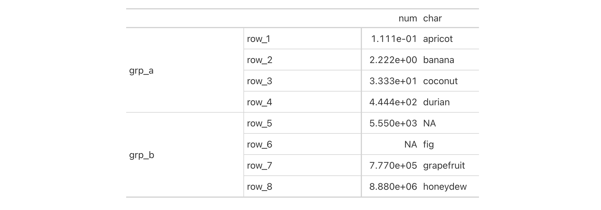
Or target specific stub columns (1 = rightmost, 2 = second from right):
exibble |>
dplyr::select(num, char, row, group) |>
gt(rowname_col = c("group", "row")) |>
cols_width(
stub(1) ~ px(70), # Rightmost stub column (row)
stub(2) ~ px(200), # Second stub column (group)
everything() ~ px(100)
)
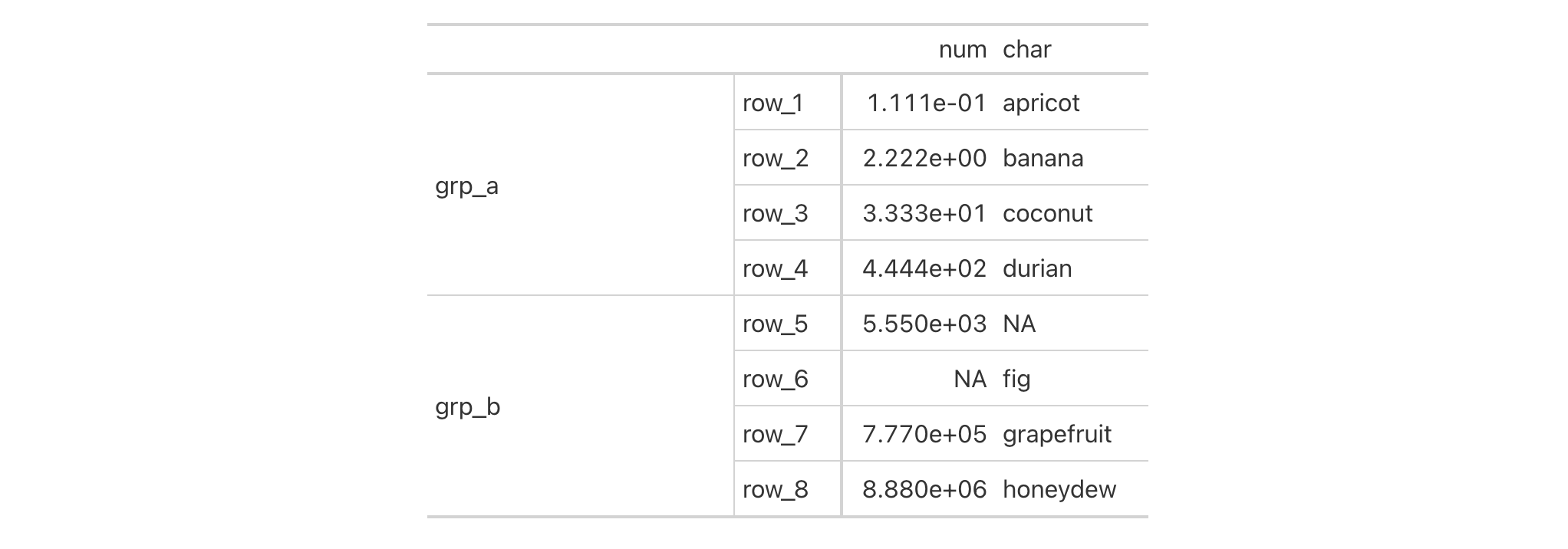
Function ID
8-10
Function Introduced
v0.8.0 (November 16, 2022)
See Also
Other helper functions:
adjust_luminance(),
cell_borders(),
cell_fill(),
cell_text(),
currency(),
default_fonts(),
escape_latex(),
from_column(),
google_font(),
gt_latex_dependencies(),
html(),
latex(),
md(),
nanoplot_options(),
pct(),
px(),
random_id(),
row_group(),
system_fonts(),
unit_conversion()
Substitute large values in the table body
Description
Wherever there are numerical data that are very large in value, replacement
text may be better for explanatory purposes. sub_large_vals() allows for
this replacement through specification of a threshold, a large_pattern,
and the sign (positive or negative) of the values to be considered.
Usage
sub_large_vals( data, columns = everything(), rows = everything(), threshold = 1e+12, large_pattern = ">={x}", sign = "+" )sub_large_vals( data, columns = everything(), rows = everything(), threshold = 1e+12, large_pattern = ">={x}", sign = "+" )
Arguments
data |
The gt table data object
This is the gt table object that is commonly created through use of the
|
columns |
Columns to target
The columns to which substitution operations are constrained. Can either
be a series of column names provided in |
rows |
Rows to target
In conjunction with |
threshold |
Threshold value
The threshold value with which values should be considered large enough for replacement. |
large_pattern |
Pattern specification for large values
The pattern text to be used in place of the suitably large values in the rendered table. |
sign |
Consider positive or negative values?
The sign of the numbers to be considered in the replacement. By default, we
only consider positive values ( |
Value
An object of class gt_tbl.
Examples
Let's generate a simple, single-column tibble that contains an assortment of values that could potentially undergo some substitution.
tbl <- dplyr::tibble(num = c(0, NA, 10^(8:14))) tbl #> # A tibble: 9 x 1 #> num #> <dbl> #> 1 0 #> 2 NA #> 3 1e 8 #> 4 1e 9 #> 5 1e10 #> 6 1e11 #> 7 1e12 #> 8 1e13 #> 9 1e14
The tbl object contains a variety of larger numbers and some might be
larger enough to reformat with a threshold value. With sub_large_vals() we
can do just that:
tbl |> gt() |> fmt_number(columns = num) |> sub_large_vals()

Large negative values can also be handled but they are handled specially by
the sign parameter. Setting that to "-" will format only the large values
that are negative. Notice that with the default large_pattern value of
">={x}" the ">=" is automatically changed to "<=".
tbl |> dplyr::mutate(num = -num) |> gt() |> fmt_number(columns = num) |> sub_large_vals(sign = "-")

You don't have to settle with the default threshold value or the default
replacement pattern (in large_pattern). This can be changed and the
"{x}" in large_pattern (which uses the threshold value) can even be
omitted.
tbl |>
gt() |>
fmt_number(columns = num) |>
sub_large_vals(
threshold = 5E10,
large_pattern = "hugemongous"
)

Function ID
3-35
Function Introduced
v0.6.0 (May 24, 2022)
See Also
Other data formatting functions:
data_color(),
fmt(),
fmt_auto(),
fmt_bins(),
fmt_bytes(),
fmt_chem(),
fmt_country(),
fmt_currency(),
fmt_date(),
fmt_datetime(),
fmt_duration(),
fmt_email(),
fmt_engineering(),
fmt_flag(),
fmt_fraction(),
fmt_icon(),
fmt_image(),
fmt_index(),
fmt_integer(),
fmt_markdown(),
fmt_number(),
fmt_number_si(),
fmt_partsper(),
fmt_passthrough(),
fmt_percent(),
fmt_roman(),
fmt_scientific(),
fmt_spelled_num(),
fmt_tf(),
fmt_time(),
fmt_units(),
fmt_url(),
sub_missing(),
sub_small_vals(),
sub_values(),
sub_zero()
Substitute missing values in the table body
Description
Wherever there is missing data (i.e., NA values) customizable content may
present better than the standard NA text that would otherwise appear.
sub_missing() allows for this replacement through its missing_text
argument (where an em dash serves as the default).
Usage
sub_missing( data, columns = everything(), rows = everything(), missing_text = "---" )sub_missing( data, columns = everything(), rows = everything(), missing_text = "---" )
Arguments
data |
The gt table data object
This is the gt table object that is commonly created through use of the
|
columns |
Columns to target
The columns to which substitution operations are constrained. Can either
be a series of column names provided in |
rows |
Rows to target
In conjunction with |
missing_text |
Replacement text for
The text to be used in place of |
Value
An object of class gt_tbl.
Examples
Use select columns from the exibble dataset to create a gt table. The
NA values in different columns (here, we are using column indices in
columns) will be given two variations of replacement text with two separate
calls of sub_missing().
exibble |>
dplyr::select(-row, -group) |>
gt() |>
sub_missing(
columns = 1:2,
missing_text = "missing"
) |>
sub_missing(
columns = 4:7,
missing_text = "nothing"
)

Function ID
3-32
Function Introduced
v0.6.0 (May 24, 2022)
See Also
Other data formatting functions:
data_color(),
fmt(),
fmt_auto(),
fmt_bins(),
fmt_bytes(),
fmt_chem(),
fmt_country(),
fmt_currency(),
fmt_date(),
fmt_datetime(),
fmt_duration(),
fmt_email(),
fmt_engineering(),
fmt_flag(),
fmt_fraction(),
fmt_icon(),
fmt_image(),
fmt_index(),
fmt_integer(),
fmt_markdown(),
fmt_number(),
fmt_number_si(),
fmt_partsper(),
fmt_passthrough(),
fmt_percent(),
fmt_roman(),
fmt_scientific(),
fmt_spelled_num(),
fmt_tf(),
fmt_time(),
fmt_units(),
fmt_url(),
sub_large_vals(),
sub_small_vals(),
sub_values(),
sub_zero()
Substitute small values in the table body
Description
Wherever there is numerical data that are very small in value, replacement
text may be better for explanatory purposes. sub_small_vals() allows for
this replacement through specification of a threshold, a small_pattern,
and the sign of the values to be considered. The substitution will occur for
those values found to be between 0 and the threshold value. This is
possible for small positive and small negative values (this can be explicitly
set by the sign option). Note that the interval does not include the 0 or
the threshold value. Should you need to include zero values, use
sub_zero().
Usage
sub_small_vals( data, columns = everything(), rows = everything(), threshold = 0.01, small_pattern = if (sign == "+") "<{x}" else md("<*abs*(-{x})"), sign = "+" )sub_small_vals( data, columns = everything(), rows = everything(), threshold = 0.01, small_pattern = if (sign == "+") "<{x}" else md("<*abs*(-{x})"), sign = "+" )
Arguments
data |
The gt table data object
This is the gt table object that is commonly created through use of the
|
columns |
Columns to target
The columns to which substitution operations are constrained. Can either
be a series of column names provided in |
rows |
Rows to target
In conjunction with |
threshold |
Threshold value
The threshold value with which values should be considered small enough for replacement. |
small_pattern |
Pattern specification for small values
The pattern text to be used in place of the suitably small values in the rendered table. |
sign |
Consider positive or negative values?
The sign of the numbers to be considered in the replacement. By default, we
only consider positive values ( |
Value
An object of class gt_tbl.
Examples
Let's generate a simple, single-column tibble that contains an assortment of values that could potentially undergo some substitution.
tbl <- dplyr::tibble(num = c(10^(-4:2), 0, NA)) tbl #> # A tibble: 9 x 1 #> num #> <dbl> #> 1 0.0001 #> 2 0.001 #> 3 0.01 #> 4 0.1 #> 5 1 #> 6 10 #> 7 100 #> 8 0 #> 9 NA
The tbl contains a variety of smaller numbers and some might be small
enough to reformat with a threshold value. With sub_small_vals() we can
do just that:
tbl |> gt() |> fmt_number(columns = num) |> sub_small_vals()

Small and negative values can also be handled but they are handled specially
by the sign parameter. Setting that to "-" will format only the small,
negative values.
tbl |> dplyr::mutate(num = -num) |> gt() |> fmt_number(columns = num) |> sub_small_vals(sign = "-")

You don't have to settle with the default threshold value or the default
replacement pattern (in small_pattern). This can be changed and the
"{x}" in small_pattern (which uses the threshold value) can even be
omitted.
tbl |>
gt() |>
fmt_number(columns = num) |>
sub_small_vals(
threshold = 0.0005,
small_pattern = "smol"
)

Function ID
3-34
Function Introduced
v0.6.0 (May 24, 2022)
See Also
Other data formatting functions:
data_color(),
fmt(),
fmt_auto(),
fmt_bins(),
fmt_bytes(),
fmt_chem(),
fmt_country(),
fmt_currency(),
fmt_date(),
fmt_datetime(),
fmt_duration(),
fmt_email(),
fmt_engineering(),
fmt_flag(),
fmt_fraction(),
fmt_icon(),
fmt_image(),
fmt_index(),
fmt_integer(),
fmt_markdown(),
fmt_number(),
fmt_number_si(),
fmt_partsper(),
fmt_passthrough(),
fmt_percent(),
fmt_roman(),
fmt_scientific(),
fmt_spelled_num(),
fmt_tf(),
fmt_time(),
fmt_units(),
fmt_url(),
sub_large_vals(),
sub_missing(),
sub_values(),
sub_zero()
Substitute targeted values in the table body
Description
Should you need to replace specific cell values with custom text,
sub_values() can be good choice. We can target cells for replacement
through value, regex, and custom matching rules.
Usage
sub_values( data, columns = everything(), rows = everything(), values = NULL, pattern = NULL, fn = NULL, replacement = NULL, escape = TRUE )sub_values( data, columns = everything(), rows = everything(), values = NULL, pattern = NULL, fn = NULL, replacement = NULL, escape = TRUE )
Arguments
data |
The gt table data object
This is the gt table object that is commonly created through use of the
|
columns |
Columns to target
The columns to which substitution operations are constrained. Can either
be a series of column names provided in |
rows |
Rows to target
In conjunction with |
values |
Values to match on
The specific value or values that should be replaced with a |
pattern |
Regex pattern to match with
A regex pattern that can target solely those values in |
fn |
Function to return logical values
A supplied function that operates on |
replacement |
Replacement value for matches
The replacement value for any cell values matched by either |
escape |
Text escaping
An option to escape replacement text according to the final output format
of the table. For example, if a LaTeX table is to be generated then LaTeX
escaping would be performed on the replacements during rendering. By
default this is set to |
Value
An object of class gt_tbl.
Examples
Let's create an input table with three columns. This contains an assortment
of values that could potentially undergo some substitution via
sub_values().
tbl <-
dplyr::tibble(
num_1 = c(-0.01, 74, NA, 0, 500, 0.001, 84.3),
int_1 = c(1L, -100000L, 800L, 5L, NA, 1L, -32L),
lett = LETTERS[1:7]
)
tbl
#> # A tibble: 7 x 3
#> num_1 int_1 lett
#> <dbl> <int> <chr>
#> 1 -0.01 1 A
#> 2 74 -100000 B
#> 3 NA 800 C
#> 4 0 5 D
#> 5 500 NA E
#> 6 0.001 1 F
#> 7 84.3 -32 G
Values in the table body cells can be replaced by specifying which values
should be replaced (in values) and what the replacement value should be.
It's okay to search for numerical or character values across all columns and
the replacement value can also be of the numeric or character types.
tbl |> gt() |> sub_values(values = c(74, 500), replacement = 150) |> sub_values(values = "B", replacement = "Bee") |> sub_values(values = 800, replacement = "Eight hundred")

We can also use the pattern argument to target cell values for replacement
in character-based columns.
tbl |> gt() |> sub_values(pattern = "A|C|E", replacement = "Ace")

For the most flexibility, it's best to use the fn argument. With that you
need to ensure that the function you provide will return a logical vector
when invoked on a column of cell values, taken as x (and, the length of
that vector must match the length of x).
tbl |>
gt() |>
sub_values(
fn = function(x) x >= 0 & x < 50,
replacement = "Between 0 and 50"
)

Function ID
3-36
Function Introduced
v0.8.0 (November 16, 2022)
See Also
Other data formatting functions:
data_color(),
fmt(),
fmt_auto(),
fmt_bins(),
fmt_bytes(),
fmt_chem(),
fmt_country(),
fmt_currency(),
fmt_date(),
fmt_datetime(),
fmt_duration(),
fmt_email(),
fmt_engineering(),
fmt_flag(),
fmt_fraction(),
fmt_icon(),
fmt_image(),
fmt_index(),
fmt_integer(),
fmt_markdown(),
fmt_number(),
fmt_number_si(),
fmt_partsper(),
fmt_passthrough(),
fmt_percent(),
fmt_roman(),
fmt_scientific(),
fmt_spelled_num(),
fmt_tf(),
fmt_time(),
fmt_units(),
fmt_url(),
sub_large_vals(),
sub_missing(),
sub_small_vals(),
sub_zero()
Substitute zero values in the table body
Description
Wherever there is numerical data that are zero in value, replacement text may
be better for explanatory purposes. sub_zero() allows for this replacement
through its zero_text argument.
Usage
sub_zero(data, columns = everything(), rows = everything(), zero_text = "nil")sub_zero(data, columns = everything(), rows = everything(), zero_text = "nil")
Arguments
data |
The gt table data object
This is the gt table object that is commonly created through use of the
|
columns |
Columns to target
The columns to which substitution operations are constrained. Can either
be a series of column names provided in |
rows |
Rows to target
In conjunction with |
zero_text |
Replacement text for zero values
The text to be used in place of zero values in the rendered table. We can
optionally use |
Value
An object of class gt_tbl.
Examples
Let's generate a simple, single-column tibble that contains an assortment of values that could potentially undergo some substitution.
tbl <- dplyr::tibble(num = c(10^(-1:2), 0, 0, 10^(4:6))) tbl #> # A tibble: 9 x 1 #> num #> <dbl> #> 1 0.1 #> 2 1 #> 3 10 #> 4 100 #> 5 0 #> 6 0 #> 7 10000 #> 8 100000 #> 9 1000000
With this table, the zero values in will be given replacement text with a
single call of sub_zero().
tbl |> gt() |> fmt_number(columns = num) |> sub_zero()

Function ID
3-33
Function Introduced
v0.6.0 (May 24, 2022)
See Also
Other data formatting functions:
data_color(),
fmt(),
fmt_auto(),
fmt_bins(),
fmt_bytes(),
fmt_chem(),
fmt_country(),
fmt_currency(),
fmt_date(),
fmt_datetime(),
fmt_duration(),
fmt_email(),
fmt_engineering(),
fmt_flag(),
fmt_fraction(),
fmt_icon(),
fmt_image(),
fmt_index(),
fmt_integer(),
fmt_markdown(),
fmt_number(),
fmt_number_si(),
fmt_partsper(),
fmt_passthrough(),
fmt_percent(),
fmt_roman(),
fmt_scientific(),
fmt_spelled_num(),
fmt_tf(),
fmt_time(),
fmt_units(),
fmt_url(),
sub_large_vals(),
sub_missing(),
sub_small_vals(),
sub_values()
Add summary columns using aggregation functions
Description
The summary_columns() function adds one or more computed columns to a table
by aggregating values across selected columns within each row. This is the
horizontal counterpart to summary_rows(), which aggregates down columns to
create summary rows. Common use cases include calculating row totals, row
averages, or other row-wise statistics.
Summary columns are computed immediately when the function is called and are
added to the table's data as regular columns. This means they can be
referenced in subsequent gt operations like cols_move(), fmt_number(),
tab_style(), or even in other computed columns via cols_add().
You can create a single summary column or multiple columns at once by
providing a list of aggregation functions. The functions can be any R
expression that takes a vector of values and returns a single value (like
sum(), mean(), max(), min(), etc.). Column names and labels can be
auto-generated from function names or explicitly specified.
Usage
summary_columns( data, columns = everything(), fns = NULL, new_col_names = NULL, new_col_labels = NULL, fmt = NULL, side = c("right", "left"), missing_text = "---" )summary_columns( data, columns = everything(), fns = NULL, new_col_names = NULL, new_col_labels = NULL, fmt = NULL, side = c("right", "left"), missing_text = "---" )
Arguments
data |
The gt table data object
This is the gt table object that is commonly created through use of the
|
columns |
Columns to aggregate
The columns to aggregate across for each row. Can either be a series of
column names provided in |
fns |
Aggregation Expression(s)
One or more functions used for aggregation. For a single summary column,
provide a single function as a formula (e.g., |
new_col_names |
Names for new summary columns
Optional names for the new summary columns. Can provide one name for a
single summary column, or multiple names (must match the length of |
new_col_labels |
Labels for new summary columns
Optional labels for the new summary column headers. Can provide one label
for a single column, or multiple labels (must match the length of |
fmt |
Formatting expression
An optional formatting expression in formula form. The RHS of |
side |
Side used for placement of summary column
Should the summary column be placed on the |
missing_text |
Replacement text for
The text to be used in place of |
Value
An object of class gt_tbl.
Examples
Use a subset of the countrypops dataset to create a gt table. Add a
summary column that computes the average annual change using
summary_columns().
countrypops |>
arrange(country_name, year) |>
group_by(country_name, country_code_2) |>
summarize(
pop_1960 = first(population),
pop_2024 = last(population),
years = n(),
.groups = "drop"
) |>
filter(!is.na(pop_1960), !is.na(pop_2024)) |>
mutate(total_change = pop_2024 - pop_1960) |>
slice_max(total_change, n = 5) |>
select(country_name, country_code_2, pop_1960, pop_2024, years) |>
gt() |>
summary_columns(
columns = c(pop_1960, pop_2024, years),
fns = ~ (.[2] - .[1]) / (.[3] - 1),
new_col_names = "avg_annual_change",
new_col_labels = md("**Avg. Annual Change**") # No list() needed!
) |>
cols_hide(columns = c(pop_1960, pop_2024, years)) |>
fmt_integer() |>
cols_label(
country_name = "Country",
country_code_2 = "Code"
) |>
tab_header(
title = "Top 5 Countries by Population Growth",
subtitle = "Average annual population change (1960-2024)"
)

Function ID
6-6
Function Introduced
v1.2.0 (December 16, 2025)
See Also
Other row addition/modification functions:
grand_summary_rows(),
row_group_order(),
row_order(),
rows_add(),
rows_hide(),
rows_unhide(),
summary_rows()
Add group-wise summary rows using aggregation functions
Description
Add summary rows to one or more row groups by using the table data and any
suitable aggregation functions. Multiple summary rows can be added for
selected groups via expressions given to fns. You can selectively format
the values in the resulting summary cells by use of formatting expressions in
fmt.
Usage
summary_rows( data, groups = everything(), columns = everything(), fns = NULL, fmt = NULL, side = c("bottom", "top"), missing_text = "---", formatter = NULL, ... )summary_rows( data, groups = everything(), columns = everything(), fns = NULL, fmt = NULL, side = c("bottom", "top"), missing_text = "---", formatter = NULL, ... )
Arguments
data |
The gt table data object
This is the gt table object that is commonly created through use of the
|
groups |
Specification of row group IDs
The row groups to which targeting operations are constrained. Can either be
a series of row group ID values provided in |
columns |
Columns to target
The columns for which the summaries should be calculated. Can either
be a series of column names provided in |
fns |
Aggregation Expressions
Functions used for aggregations. This can include base functions like
|
fmt |
Formatting expressions
Formatting expressions in formula form. The RHS of |
side |
Side used for placement of summary rows
Should the summary rows be placed at the |
missing_text |
Replacement text for
The text to be used in place of |
formatter |
Deprecated Formatting function
Deprecated, please use |
... |
Deprecated Formatting arguments
Deprecated (along with |
Value
An object of class gt_tbl.
Using columns to target column data for aggregation
Targeting of column data for which aggregates should be generated is done
through the columns argument. We can declare column names in c() (with
bare column names or names in quotes) or we can use
tidyselect-style expressions. This can be as basic as supplying a select
helper like starts_with(), or, providing a more complex incantation like
where(~ is.numeric(.x) & max(.x, na.rm = TRUE) > 1E6)
which targets numeric columns that have a maximum value greater than
1,000,000 (excluding any NAs from consideration).
By default all columns are selected (with the everything() default). This
default may be not what's needed unless all columns can undergo useful
aggregation by expressions supplied in fns.
Aggregation expressions for fns
There are a number of ways to express how an aggregation should work for
each summary row. In addition to that, we have the ability to pass important
information such as the summary row ID value and its label (the former
necessary for targeting within tab_style() or tab_footnote() and the
latter used for display in the rendered table). Here are a number of
instructive examples for how to supply such expressions.
Double-sided formula with everything supplied
We can be explicit and provide a double-sided formula (in the form
<LHS> ~ <RHS>) that expresses everything about a summary row. That is, it
has an aggregation expression (where . represents the data in the
focused column). Here's an example:
list(id = "minimum", label = "min") ~ min(., na.rm = TRUE)
The left side (the list) contains named elements that identify the id and
label for the summary row. The right side has an expression for obtaining
a minimum value (dropping NA values in the calculation).
The list() can be replaced with c() but the advantage of a list is
allowing the use of the md() and html() helper functions. The above
example can be written as:
list(id = "minimum", label = md("**Minimum**")) ~ min(., na.rm = TRUE)
and we can have that label value interpreted as Markdown text.
Function names in quotes
With fns = "min" we get the equivalent of the fuller expression:
list(id = "min", label = "min") ~ min(., na.rm = TRUE)
For sake of convenience, common aggregation functions with the na.rm
argument will be rewritten with the na.rm = TRUE option. These functions
are: "min", "max", "mean", "median", "sd", and "sum".
Should you need to specify multiple aggregation functions in this way (giving
you multiple summary rows), use c() or list().
RHS formula expressions
With fns = ~ min(.) or fns = list(~ min(.)), gt will use the function
name as the id and label. The expansion of this shorthand to full form
looks like this:
list(id = "min", label = "min") ~ min(.)
The RHS expression is kept as written and the name portion is both the id
and the label.
Named vector or list with RHS formula expression
Using fns = c(minimum = ~ min(.)) or fns = list(minimum = ~ min(.))
expands to this:
list(id = "minimum", label = "minimum") ~ min(.)
Unnamed vector or list with RHS formula expression
With fns = c("minimum", "min") ~ min(.) or
fns = list("minimum", "min") ~ min(.) the LHS contains the label and id
values and, importantly, the order is label first and id second. This can
be rewritten as:
list(id = "min", label = "minimum") ~ min(.)
If the vector or list is partially named, gt has enough to go on to
disambiguate the unnamed element. So with
fns = c("minimum", label = "min") ~ min(.), "min" is indeed the label
and "minimum" is taken as the id value.
A fully named list with three specific elements
We can avoid using a formula if we are satisfied with the default options of
a function (except some of those functions with the na.rm options, see
above). Instead, a list with the named elements id, label, and fn could
be used. It can look like this:
fns = list(id = "mean_id", label = "average", fn = "mean")
which translates to
list(id = "mean_id", label = "average") ~ mean(., na.rm = TRUE)
Formatting expressions for fmt
Given that we are generating new data in a table, we might also want to
take the opportunity to format those new values right away. We can do this
in the fmt argument, either with a single expression or a number of them
in a list.
Formatting cells across all groups
We can supply a one-sided (RHS only) or two-sided expression (targeting
groups) to fmt, and, several can be provided in a list. The RHS will always
contain an expression that uses a formatting function (e.g., fmt_number(),
fmt_currency(), etc.) and it must contain an initial . that stands for
the data object. If performing numeric formatting on all columns in the new
summary rows, it might look something like this:
fmt = ~ fmt_number(., decimals = 1, use_seps = FALSE)
We can use the columns and rows arguments that are available in every
formatting function. This allows us to format only a subset of columns or
rows. Summary rows can be targeted by using their ID values and these are
settable within expressions given to fns (see the Aggregation expressions
for fns section for details on this). Here's an example with hypothetical
column and row names:
fmt = ~ fmt_number(., columns = num, rows = "mean", decimals = 3)
Formatting cells in specific groups
A two-sided expression is needed for targeting the formatting directives to
specific summary row groups. In this format, the LHS should contain an
expression that resolves to a set of available groups. We can use a single
row group name in quotes, several of those in a vector, or a select helper
expression like starts_with() or matches().
In a situation where summary rows were generated across the row groups named
"group_1", "group_2", and "group_3", we could format all summary cells
in "group_2" with the following:
fmt = "group_2" ~ fmt_number(., decimals = 1, use_seps = FALSE)
If you wanted to target the latter two groups, this can be done:
fmt = matches("2|3") ~ fmt_number(., decimals = 1, use_seps = FALSE)
Should you need to target a single cell, the LHS expression for group
targeting could be paired with single values for columns and rows on the
RHS formatting expression. Like this:
fmt = "group_1" ~ fmt_number(., columns = num, rows = "mean")
Extraction of summary rows
Should we need to obtain the summary data for external purposes,
extract_summary() can be used with a gt_tbl object where summary rows
were added via summary_rows() or grand_summary_rows().
Examples
Use a modified version of sp500 dataset to create a gt table with row
groups and row labels. Create the summary rows labeled min, max, and
avg by row group (where each each row group is a week number) with
summary_rows().
sp500 |>
dplyr::filter(date >= "2015-01-05" & date <= "2015-01-16") |>
dplyr::arrange(date) |>
dplyr::mutate(week = paste0("W", strftime(date, format = "%V"))) |>
dplyr::select(-adj_close, -volume) |>
gt(
rowname_col = "date",
groupname_col = "week"
) |>
summary_rows(
fns = list(
"min",
"max",
list(label = "avg", fn = "mean")
),
fmt = ~ fmt_number(., use_seps = FALSE)
)
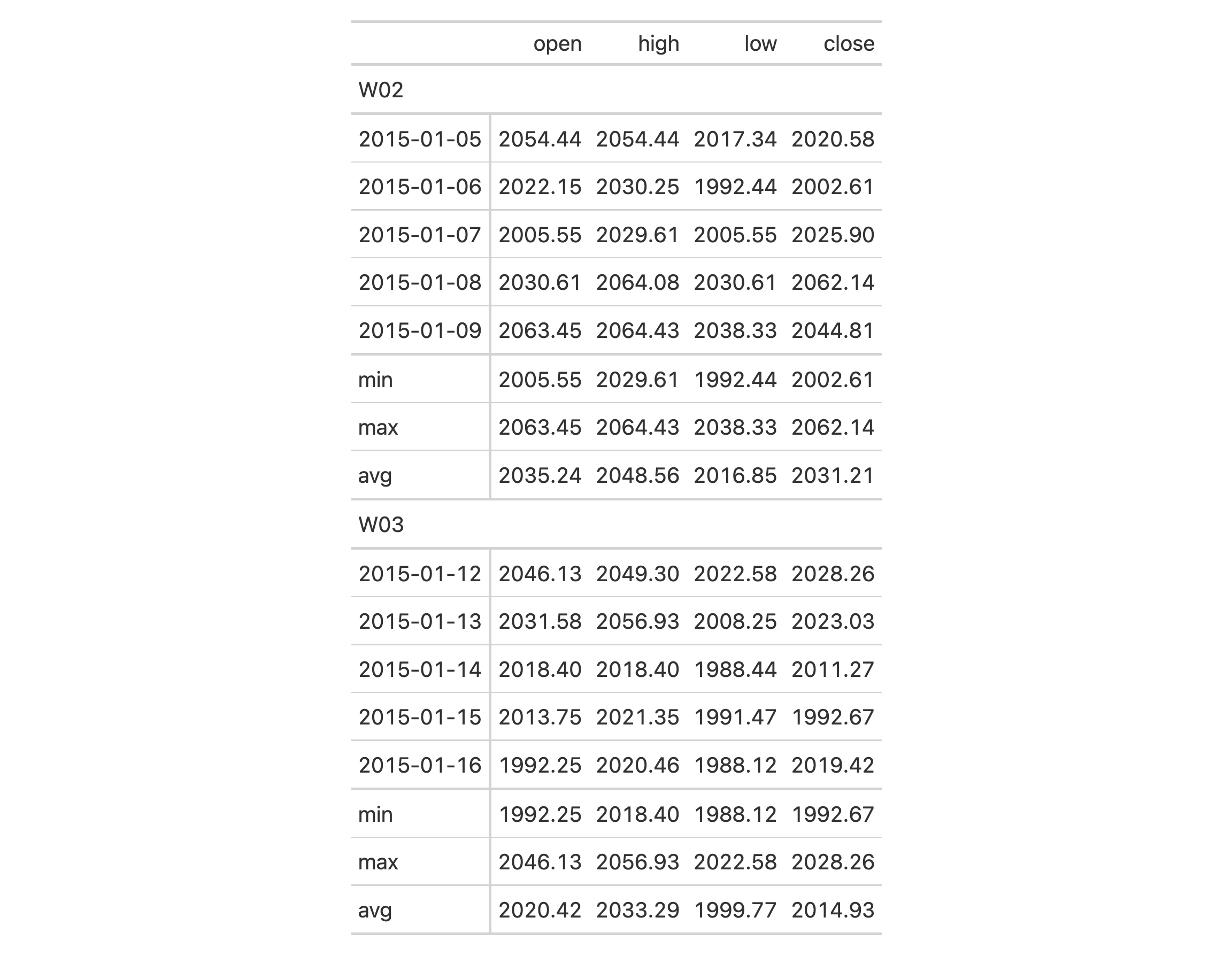
Using the countrypops dataset, let's process that a bit before giving it
to gt. We can create a summary rows with totals that appear at the top of
each row group (with side = "top"). We can define the aggregation with a
list that contains parameters for the summary row label (md("**ALL**")),
the shared ID value of those rows across groups ("totals"), and the
aggregation function (expressed as "sum", which gt recognizes as the
sum() function). To top it all off, we'll add background fills to the
summary rows with tab_style().
countrypops |>
dplyr::filter(
country_code_2 %in% c("BR", "RU", "IN", "CN", "FR", "DE", "IT", "GB")
) |>
dplyr::filter(year %% 10 == 0) |>
dplyr::select(country_name, year, population) |>
tidyr::pivot_wider(names_from = year, values_from = population) |>
gt(rowname_col = "country_name") |>
tab_row_group(
label = md("*BRIC*"),
rows = c("Brazil", "Russia", "India", "China"),
id = "bric"
) |>
tab_row_group(
label = md("*Big Four*"),
rows = c("France", "Germany", "Italy", "United Kingdom"),
id = "big4"
) |>
row_group_order(groups = c("bric", "big4")) |>
tab_stub_indent(rows = everything()) |>
tab_header(title = "Populations of the BRIC and Big Four Countries") |>
tab_spanner(columns = everything(), label = "Year") |>
fmt_number(n_sigfig = 3, suffixing = TRUE) |>
summary_rows(
fns = list(label = md("**ALL**"), id = "totals", fn = "sum"),
fmt = ~ fmt_number(., n_sigfig = 3, suffixing = TRUE),
side = "top"
) |>
tab_style(
locations = cells_summary(),
style = cell_fill(color = "lightblue" |> adjust_luminance(steps = +1))
)

Function ID
6-1
Function Introduced
v0.2.0.5 (March 31, 2020)
See Also
Other row addition/modification functions:
grand_summary_rows(),
row_group_order(),
row_order(),
rows_add(),
rows_hide(),
rows_unhide(),
summary_columns()
Get a themed font stack that works well across systems
Description
A font stack can be obtained from system_fonts() using one of various
keywords such as "system-ui", "old-style", and "humanist" (there are 15
in total) representing a themed set of fonts. These sets comprise a font
family that has been tested to work across a wide range of computer systems.
This is useful when specifying font values in cell_text()
(itself used inside tab_style()). If using opt_table_font(), we can
invoke this function in its stack argument.
Usage
system_fonts(name)system_fonts(name)
Arguments
name |
Name of font stack
The name of a font stack. Must be drawn from the set of |
Value
A character vector of font names.
The font stacks and the individual fonts used by platform
System UI ("system-ui")
font-family: system-ui, sans-serif;
The operating system interface's default typefaces are known as system UI fonts. They contain a variety of font weights, are quite readable at small sizes, and are perfect for UI elements. These typefaces serve as a great starting point for text in data tables and so this font stack is the default for gt.
Transitional ("transitional")
font-family: Charter, 'Bitstream Charter', 'Sitka Text', Cambria, serif;
The Enlightenment saw the development of transitional typefaces, which combine Old Style and Modern typefaces. Times New Roman, a transitional typeface created for the Times of London newspaper, is among the most well-known instances of this style.
Old Style ("old-style")
font-family: 'Iowan Old Style', 'Palatino Linotype', 'URW Palladio L', P052, serif;
Old style typefaces were created during the Renaissance and are distinguished by diagonal stress, a lack of contrast between thick and thin strokes, and rounded serifs. Garamond is among the most well-known instances of an antique typeface.
Humanist ("humanist")
font-family: Seravek, 'Gill Sans Nova', Ubuntu, Calibri, 'DejaVu Sans', source-sans-pro, sans-serif;
Low contrast between thick and thin strokes and organic, calligraphic forms are traits of humanist typefaces. These typefaces, which draw their inspiration from Renaissance calligraphy, are frequently regarded as being more readable and easier to read than other sans serif typefaces.
Geometric Humanist ("geometric-humanist")
font-family: Avenir, Montserrat, Corbel, 'URW Gothic', source-sans-pro, sans-serif;
Clean, geometric forms and consistent stroke widths are characteristics of geometric humanist typefaces. These typefaces, which are frequently used for headlines and other display purposes, are frequently thought to be contemporary and slick in appearance. A well-known example of this classification is Futura.
Classical Humanist ("classical-humanist")
font-family: Optima, Candara, 'Noto Sans', source-sans-pro, sans-serif;
The way the strokes gradually widen as they approach the stroke terminals without ending in a serif is what distinguishes classical humanist typefaces. The stone carving on Renaissance-era tombstones and classical Roman capitals served as inspiration for these typefaces.
Neo-Grotesque ("neo-grotesque")
font-family: Inter, Roboto, 'Helvetica Neue', 'Arial Nova', 'Nimbus Sans', Arial, sans-serif;
Neo-grotesque typefaces are a form of sans serif that originated in the late 19th and early 20th centuries. They are distinguished by their crisp, geometric shapes and regular stroke widths. Helvetica is among the most well-known examples of a Neo-grotesque typeface.
Monospace Slab Serif ("monospace-slab-serif")
font-family: 'Nimbus Mono PS', 'Courier New', monospace;
Monospace slab serif typefaces are distinguished by their fixed-width letters, which are the same width irrespective of their shape, and their straightforward, geometric forms. For reports, tabular work, and technical documentation, this technique is used to simulate typewriter output.
Monospace Code ("monospace-code")
font-family: ui-monospace, 'Cascadia Code', 'Source Code Pro', Menlo, Consolas, 'DejaVu Sans Mono', monospace;
Specifically created for use in programming and other technical applications, monospace code typefaces are used in these fields. These typefaces are distinguished by their clear, readable forms and monospaced design, which ensures that all letters and characters are the same width.
Industrial ("industrial")
font-family: Bahnschrift, 'DIN Alternate', 'Franklin Gothic Medium', 'Nimbus Sans Narrow', sans-serif-condensed, sans-serif;
The development of industrial typefaces began in the late 19th century and was greatly influenced by the industrial and technological advancements of the time. Industrial typefaces are distinguished by their strong sans serif letterforms, straightforward appearance, and use of geometric shapes and straight lines.
Rounded Sans ("rounded-sans")
font-family: ui-rounded, 'Hiragino Maru Gothic ProN', Quicksand, Comfortaa, Manjari, 'Arial Rounded MT', 'Arial Rounded MT Bold', Calibri, source-sans-pro, sans-serif;
The rounded, curved letterforms that define rounded typefaces give them a softer, friendlier appearance. The typeface's rounded edges give it a more natural and playful feel, making it appropriate for use in casual or kid-friendly designs. Since the 1950s, the rounded sans-serif design has gained popularity and is still frequently used in branding, graphic design, and other fields.
Slab Serif ("slab-serif")
font-family: Rockwell, 'Rockwell Nova', 'Roboto Slab', 'DejaVu Serif', 'Sitka Small', serif;
Slab Serif typefaces are distinguished by the thick, block-like serifs that appear at the ends of each letterform. Typically, these serifs are unbracketed, which means that they do not have any curved or tapered transitions to the letter's main stroke.
Antique ("antique")
font-family: Superclarendon, 'Bookman Old Style', 'URW Bookman', 'URW Bookman L', 'Georgia Pro', Georgia, serif;
Serif typefaces that were popular in the 19th century include antique typefaces, also referred to as Egyptians. They are distinguished by their thick, uniform stroke weight and block-like serifs.
Didone ("didone")
font-family: Didot, 'Bodoni MT', 'Noto Serif Display', 'URW Palladio L', P052, Sylfaen, serif;
Didone typefaces, also referred to as Modern typefaces, are distinguished by their vertical stress, sharp contrast between thick and thin strokes, and hairline serifs without bracketing. The Didone style first appeared in the late 18th century and became well-known in the early 19th century.
Handwritten ("handwritten")
font-family: 'Segoe Print', 'Bradley Hand', Chilanka, TSCu_Comic, casual, cursive;
The appearance and feel of handwriting are replicated by handwritten typefaces. Although there are a wide variety of handwriting styles, this font stack tends to use a more casual and commonplace style.
Examples
Use a subset of the sp500 dataset to create a gt table with 10 rows.
For the date column and the column labels, let's use a different font stack
(the "industrial" one). The system fonts used in this particular stack are
"Bahnschrift", "DIN Alternate", "Franklin Gothic Medium", and
"Nimbus Sans Narrow" (the generic "sans-serif-condensed" and "sans-serif"
are used if the aforementioned fonts aren't available).
sp500 |>
dplyr::slice(1:10) |>
dplyr::select(-volume, -adj_close) |>
gt() |>
fmt_currency() |>
tab_style(
style = cell_text(
font = system_fonts(name = "industrial"),
size = px(18)
),
locations = list(
cells_body(columns = date),
cells_column_labels()
)
)
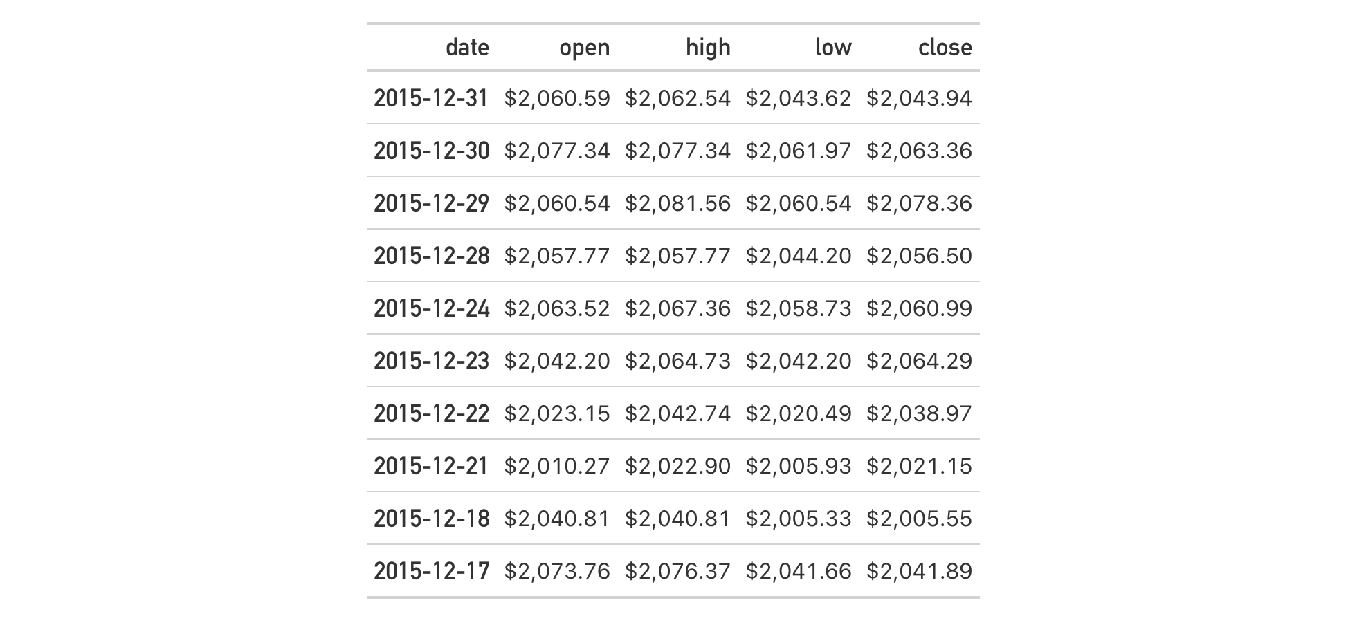
Function ID
8-33
Function Introduced
v0.9.0 (Mar 31, 2023)
See Also
Other helper functions:
adjust_luminance(),
cell_borders(),
cell_fill(),
cell_text(),
currency(),
default_fonts(),
escape_latex(),
from_column(),
google_font(),
gt_latex_dependencies(),
html(),
latex(),
md(),
nanoplot_options(),
pct(),
px(),
random_id(),
row_group(),
stub(),
unit_conversion()
Twice hourly solar zenith angles by month & latitude
Description
This dataset contains solar zenith angles (in degrees, with the range of 0-90) every half hour from 04:00 to 12:00, true solar time. This set of values is calculated on the first of every month for 4 different northern hemisphere latitudes. For determination of afternoon values, the presented tabulated values are symmetric about noon.
Usage
szasza
Format
A tibble with 816 rows and 4 variables:
- latitude
-
The latitude in decimal degrees for the observations.
- month
-
The measurement month. All calculations where conducted for the first day of each month.
- tst
-
The true solar time at the given
latitudeand date (first ofmonth) for which the solar zenith angle is calculated. - sza
-
The solar zenith angle in degrees, where
NAs indicate that sunrise hadn't yet occurred by thetstvalue.
Details
The solar zenith angle (SZA) is one measure that helps to describe the sun's path across the sky. It's defined as the angle of the sun relative to a line perpendicular to the earth's surface. It is useful to calculate the SZA in relation to the true solar time. True solar time relates to the position of the sun with respect to the observer, which is different depending on the exact longitude. For example, two hours before the sun crosses the meridian (the highest point it would reach that day) corresponds to a true solar time of 10 a.m. The SZA has a strong dependence on the observer's latitude. For example, at a latitude of 50 degrees N at the start of January, the noontime SZA is 73.0 but a different observer at 20 degrees N would measure the noontime SZA to be 43.0 degrees.
Dataset ID and Badge
DATA-2

Dataset Introduced
v0.2.0.5 (March 31, 2020)
See Also
Other datasets:
constants,
countrypops,
exibble,
films,
gibraltar,
gtcars,
illness,
metro,
nuclides,
peeps,
photolysis,
pizzaplace,
reactions,
rx_addv,
rx_adsl,
sp500,
towny
Examples
dplyr::glimpse(sza)dplyr::glimpse(sza)
Add a table caption
Description
Add a caption to a gt table, which is handled specially for a table within an R Markdown, Quarto, or bookdown context. The addition of captions makes tables cross-referencing across the containing document. The caption location (i.e., top, bottom, margin) is handled at the document level in each of these systems.
Usage
tab_caption(data, caption)tab_caption(data, caption)
Arguments
data |
The gt table data object
This is the gt table object that is commonly created through use of the
|
caption |
Table caption text
The table caption to use for cross-referencing in R Markdown, Quarto, or bookdown. |
Value
An object of class gt_tbl.
Examples
With three columns from the gtcars dataset, let's create a gt table.
First, we'll add a header part with tab_header(). After that, a caption is
added with tab_caption().
gtcars |>
dplyr::select(mfr, model, msrp) |>
dplyr::slice(1:5) |>
gt() |>
tab_header(
title = md("Data listing from **gtcars**"),
subtitle = md("`gtcars` is an R dataset")
) |>
tab_caption(caption = md("**gt** table example."))

Function ID
2-9
Function Introduced
v0.8.0 (November 16, 2022)
See Also
Other part creation/modification functions:
tab_footnote(),
tab_header(),
tab_info(),
tab_options(),
tab_row_group(),
tab_source_note(),
tab_spanner(),
tab_spanner_delim(),
tab_stub_indent(),
tab_stubhead(),
tab_style(),
tab_style_body()
Add a table footnote
Description
tab_footnote() can make it a painless process to add a footnote to a
gt table. There are commonly two components to a footnote:
(1) a footnote mark that is attached to the targeted cell content, and (2)
the footnote text itself that is placed in the table's footer area. Each unit
of footnote text in the footer is linked to an element of text or otherwise
through the footnote mark. The footnote system in gt presents footnotes
in a way that matches the usual expectations, where:
-
footnote marks have a sequence, whether they are symbols, numbers, or letters
-
multiple footnotes can be applied to the same content (and marks are always presented in an ordered fashion)
-
footnote text in the footer is never exactly repeated, gt reuses footnote marks where needed throughout the table
-
footnote marks are ordered across the table in a consistent manner (left to right, top to bottom)
Each call of tab_footnote() will either add a different footnote to the
footer or reuse existing footnote text therein. One or more cells outside of
the footer are targeted using the cells_*() helper
functions (e.g., cells_body(), cells_column_labels(), etc.). You can
choose to not attach a footnote mark by simply not specifying anything in
the locations argument.
By default, gt will choose which side of the text to place the footnote
mark via the placement = "auto" option. You are, however, always free to
choose the placement of the footnote mark (either to the "left or "right"
of the targeted cell content).
Usage
tab_footnote( data, footnote, locations = NULL, placement = c("auto", "right", "left") )tab_footnote( data, footnote, locations = NULL, placement = c("auto", "right", "left") )
Arguments
data |
The gt table data object
This is the gt table object that is commonly created through use of the
|
footnote |
Footnote text
The text to be used in the footnote. We can optionally use |
locations |
Locations to target
The cell or set of cells to be associated with the footnote. Supplying any
of the |
placement |
Placement of the footnote mark
Where to affix footnote marks to the table content. Two options for this
are |
Value
An object of class gt_tbl.
Formatting of footnote text and marks
There are several options for controlling the formatting of the footnotes,
their marks, and related typesetting in the footer. All of these options are
available within tab_options() and a subset of these are exposed in their
own opt_*() functions.
Choosing the footnote marks
We can modify the set of footnote marks with
tab_options(..., footnotes.marks) or opt_footnote_marks(..., ). What that
argument needs is a vector that will represent the series of marks. The
series of footnote marks is recycled when its usage goes beyond the length of
the set. At each cycle, the marks are simply doubled, tripled, and so on
(e.g., * -> ** -> ***). The option exists for providing keywords for
certain types of footnote marks. The keywords are:
-
"numbers": numeric marks, they begin from1and these marks are not subject to recycling behavior (this is the default) -
"letters": minuscule alphabetic marks, internally uses thelettersvector which contains 26 lowercase letters of the Roman alphabet -
"LETTERS": majuscule alphabetic marks, using theLETTERSvector which has 26 uppercase letters of the Roman alphabet -
"standard": symbolic marks, four symbols in total -
"extended": symbolic marks, extends the standard set by adding two more symbols, making six
The symbolic marks are the: (1) Asterisk, (2) Dagger, (3) Double Dagger,
(4) Section Sign, (5) Double Vertical Line, and (6) Paragraph Sign; the
"standard" set has the first four, "extended" contains all.
Defining footnote typesetting specifications
A footnote spec consists of a string containing control characters for
formatting. They are separately defined for footnote marks beside footnote
text in the table footer (the 'spec_ftr') and for marks beside the targeted
cell content (the 'spec_ref').
Not every type of formatting makes sense for footnote marks so the specification is purposefully constrained to the following:
-
as superscript text (with the
"^"control character) or regular-sized text residing on the baseline -
bold text (with
"b"), italicized text (with"i"), or unstyled text (don't use either of the"b"or"i"control characters) -
enclosure in parentheses (use
"("/")") or square brackets (with"["/"]") -
a period following the mark (using
"."); this is most commonly used in the table footer
With the aforementioned control characters we could, for instance, format
the footnote marks to be superscript text in bold type with "^b". We might
want the marks in the footer to be regular-sized text in parentheses, so the
spec could be either "()" or "(x)" (you can optionally use "x" as a
helpful placeholder for the marks).
These options can be set either in a tab_options() call (with the
footnotes.spec_ref and footnotes.spec_ftr arguments) or with
opt_footnote_spec() (using the spec_ref or spec_ftr arguments).
Additional typesetting options for footnote text residing in the footer
Within tab_options() there are two arguments that control the typesetting
of footnotes. With footnotes.multiline, we have a setting that determines
whether each footnote will start on a new line, or, whether they are combined
into a single block of text. The default for this is TRUE, but, if FALSE
we can control the separator between consecutive footnotes with the
footnotes.sep argument. By default, this is set to a single space character
(" ").
Examples
Using a subset of the sza dataset, let's create a new gt table. The
body cells in the sza column will receive background color fills according
to their data values (with data_color()). After that, the use of
tab_footnote() lets us add a footnote to the sza column label (explaining
what the color gradient signifies).
sza |>
dplyr::filter(
latitude == 20 &
month == "jan" &
!is.na(sza)
) |>
dplyr::select(-latitude, -month) |>
gt() |>
data_color(
columns = sza,
palette = c("white", "yellow", "navyblue"),
domain = c(0, 90)
) |>
tab_footnote(
footnote = "Color indicates the solar zenith angle.",
locations = cells_column_labels(columns = sza)
)
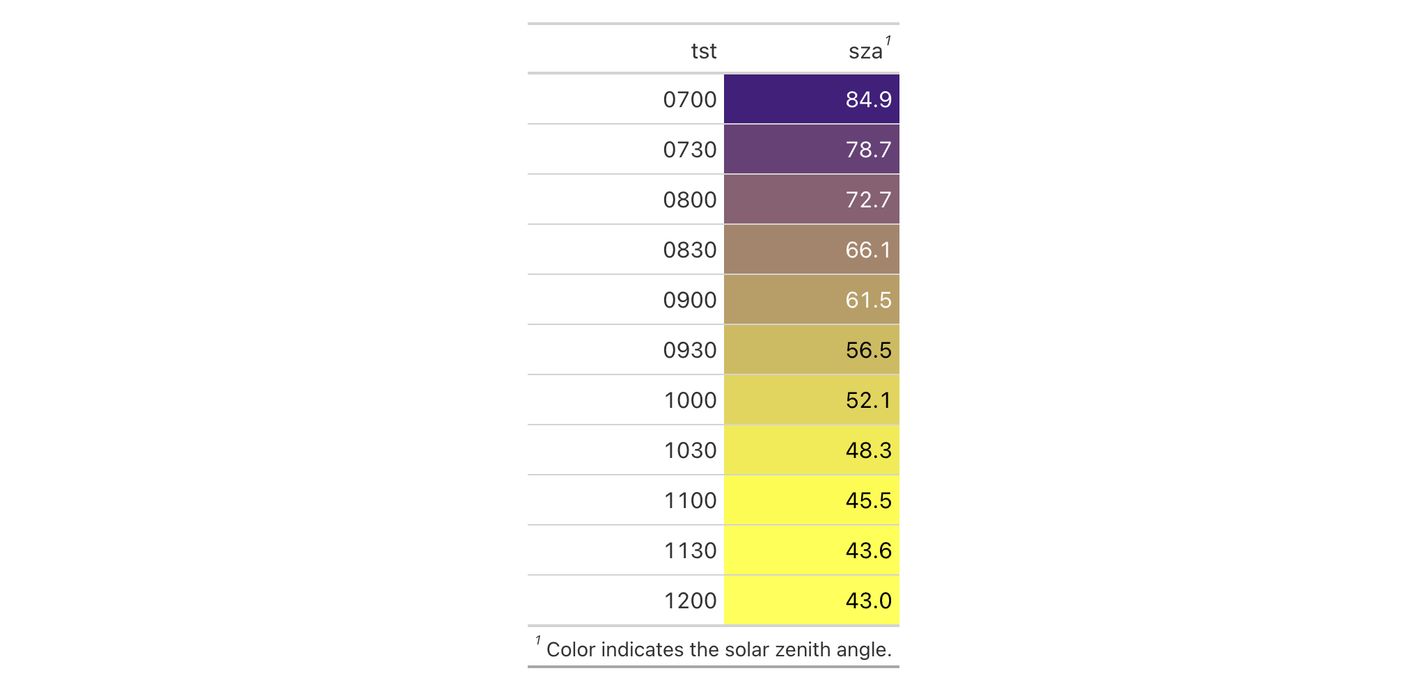
Of course, we can add more than one footnote to the table, but, we have to
use several calls of tab_footnote(). This variation of the sza table
has three footnotes: one on the "TST" column label and two on the "SZA"
column label (these were capitalized with opt_all_caps()). We will
ultimately have three calls of tab_footnote() and while the order of calls
usually doesn't matter, it does have a subtle effect here since two footnotes
are associated with the same text content (try reversing the second and third
calls and observe the effect in the footer).
sza |>
dplyr::filter(
latitude == 20 &
month == "jan" &
!is.na(sza)
) |>
dplyr::select(-latitude, -month) |>
gt() |>
opt_all_caps() |>
cols_align(align = "center") |>
cols_width(everything() ~ px(200)) |>
tab_footnote(
footnote = md("TST stands for *True Solar Time*."),
locations = cells_column_labels(columns = tst)
) |>
tab_footnote(
footnote = md("SZA stands for *Solar Zenith Angle*."),
locations = cells_column_labels(columns = sza)
) |>
tab_footnote(
footnote = "Higher Values indicate sun closer to horizon.",
locations = cells_column_labels(columns = sza)
) |>
tab_options(footnotes.multiline = FALSE)

Text in the footer (both from footnotes and also from source notes) tends to
widen the table and, by extension, all the columns within it. We can limit
that by explicitly setting column width values, which is what was done above
with cols_width(). There can also be a correspondingly large amount of
vertical space taken up by the footer since footnotes will, by default, each
start on a new line. In the above example, we used
tab_options(footnotes.multiline = FALSE) to make it so that all footer text
is contained in a single block of text.
Let's move on to another footnote-laden table, this one based on the
towny dataset. We have a header part, with a title and a subtitle. We
can choose which of these could be associated with a footnote and in this
case it is the "subtitle" (one of two options in the cells_title() helper
function). This table has a stub with row labels and some of those labels are
associated with a footnote. So long as row labels are unique, they can be
easily used as row identifiers in cells_stub(). The third footnote is
placed on the "Density" column label. Here, changing the order of the
tab_footnote() calls has no effect on the final table rendering.
towny |>
dplyr::filter(csd_type == "city") |>
dplyr::select(name, density_2021, population_2021) |>
dplyr::slice_max(population_2021, n = 10) |>
gt(rowname_col = "name") |>
tab_header(
title = md("The 10 Largest Municipalities in `towny`"),
subtitle = "Population values taken from the 2021 census."
) |>
fmt_integer() |>
cols_label(
density_2021 = "Density",
population_2021 = "Population"
) |>
tab_footnote(
footnote = "Part of the Greater Toronto Area.",
locations = cells_stub(rows = c(
"Toronto", "Mississauga", "Brampton", "Markham", "Vaughan"
))
) |>
tab_footnote(
footnote = md("Density is in terms of persons per km^2^."),
locations = cells_column_labels(columns = density_2021)
) |>
tab_footnote(
footnote = "Census results made public on February 9, 2022.",
locations = cells_title(groups = "subtitle")
) |>
tab_source_note(source_note = md(
"Data taken from the `towny` dataset (in the **gt** package)."
)) |>
opt_footnote_marks(marks = "letters")

In the above table, we elected to change the footnote marks to letters
instead of the default numbers (done through opt_footnote_marks()). A
source note was also added; this was mainly to demonstrate that source notes
will be positioned beneath footnotes in the footer section.
For our final example, let's make a relatively small table deriving from the
sp500 dataset. The set of tab_footnote() calls used here (four of them)
have minor variations that allow for interesting expressions of footnotes.
Two of the footnotes target values in the body of the table (using the
cells_body() helper function to achieve this). On numeric values that
right-aligned, gt will opt to place the footnote on the left of the
content so as to not disrupt the alignment. However, the placement argument
can be used to force the positioning of the footnote mark after the content.
We can also opt to include footnotes that have no associated footnote marks
whatsoever. This is done by not providing anything to locations. These
'markless' footnotes will precede the other footnotes in the footer section.
sp500 |>
dplyr::filter(date >= "2015-01-05" & date <="2015-01-10") |>
dplyr::select(-c(adj_close, volume, high, low)) |>
dplyr::mutate(change = close - open) |>
dplyr::arrange(date) |>
gt() |>
tab_header(title = "S&P 500") |>
fmt_date(date_style = "m_day_year") |>
fmt_currency() |>
cols_width(everything() ~ px(150)) |>
tab_footnote(
footnote = "More red days than green in this period.",
locations = cells_column_labels(columns = change)
) |>
tab_footnote(
footnote = "Lowest opening value.",
locations = cells_body(columns = open, rows = 3),
) |>
tab_footnote(
footnote = "Devastating losses on this day.",
locations = cells_body(columns = change, rows = 1),
placement = "right"
) |>
tab_footnote(footnote = "All values in USD.") |>
opt_footnote_marks(marks = "LETTERS") |>
opt_footnote_spec(spec_ref = "i[x]", spec_ftr = "x.")

Aside from changing the footnote marks to consist of "LETTERS", we've also
changed the way the marks are formatted. In our use of opt_footnote_spec(),
the spec_ref option governs the footnote marks across the table. Here, we
describe marks that are italicized and set between square brackets (with
"i[x]"). The spec_ftr argument is used for the footer representation of
the footnote marks. As described in the example with "x.", it is rendered
as a footnote mark followed by a period.
Function ID
2-7
Function Introduced
v0.2.0.5 (March 31, 2020)
See Also
Other part creation/modification functions:
tab_caption(),
tab_header(),
tab_info(),
tab_options(),
tab_row_group(),
tab_source_note(),
tab_spanner(),
tab_spanner_delim(),
tab_stub_indent(),
tab_stubhead(),
tab_style(),
tab_style_body()
Add a table header
Description
We can add a table header to the gt table with a title and even a
subtitle using tab_header(). A table header is an optional
table part that is positioned just above the column labels table part. We
have the flexibility to use Markdown or HTML formatting for the header's
title and subtitle with the md() and html() helper functions.
Usage
tab_header(data, title, subtitle = NULL, preheader = NULL)tab_header(data, title, subtitle = NULL, preheader = NULL)
Arguments
data |
The gt table data object
This is the gt table object that is commonly created through use of the
|
title |
Header title
Text to be used in the table title. We can elect to use the |
subtitle |
Header subtitle
Text to be used in the table subtitle. We can elect to use |
preheader |
RTF preheader text
Optional preheader content that is rendered above the table for RTF output. Can be supplied as a vector of text. |
Value
An object of class gt_tbl.
Examples
Let's use a small portion of the gtcars dataset to create a gt table.
A header part can be added to the table with the tab_header() function.
We'll add a title and the optional subtitle as well. With md(), we can
make sure the Markdown formatting is interpreted and transformed.
gtcars |>
dplyr::select(mfr, model, msrp) |>
dplyr::slice(1:5) |>
gt() |>
tab_header(
title = md("Data listing from **gtcars**"),
subtitle = md("`gtcars` is an R dataset")
)

If the table is intended solely as an HTML table, you could introduce your
own HTML elements into the header. You can even use the htmltools package
to help arrange and generate the HTML. Here's an example of that, where two
<div> elements are placed in a htmltools::tagList().
gtcars |>
dplyr::select(mfr, model, msrp) |>
dplyr::slice(1:5) |>
gt() |>
tab_header(
title =
htmltools::tagList(
htmltools::tags$div(
htmltools::HTML(
web_image("https://www.r-project.org/logo/Rlogo.png")
),
style = htmltools::css(`text-align` = "center")
),
htmltools::tags$div(
"Data listing from ", htmltools::tags$strong("gtcars")
)
)
)

If using HTML but doing something far simpler, we can wrap our title or
subtitle inside html() to declare that the text provided is HTML.
gtcars |>
dplyr::select(mfr, model, msrp) |>
dplyr::slice(1:5) |>
gt() |>
tab_header(
title = html("Data listing from <strong>gtcars</strong>"),
subtitle = html("From <span style='color:red;'>gtcars</span>")
)

Sometimes, aligning the heading elements to the left can improve the
presentation of a table. Here, we use the nuclides dataset to generate a
display of natural abundance values for several stable isotopes.
opt_align_table_header() is used with align = "left" to make it so the
title and subtitle are left aligned in the header area.
nuclides |>
dplyr::filter(!is.na(abundance)) |>
dplyr::filter(abundance != 1) |>
dplyr::filter(z >= 1 & z <= 8) |>
dplyr::mutate(element = paste0(element, ", **z = ", z, "**")) |>
dplyr::mutate(nuclide = gsub("[0-9]+$", "", nuclide)) |>
dplyr::select(nuclide, element, atomic_mass, abundance, abundance_uncert) |>
gt(
rowname_col = "nuclide",
groupname_col = "element",
process_md = TRUE
) |>
tab_header(
title = "Natural Abundance Values",
subtitle = md("For elements having atomic numbers from `1` to `8`.")
) |>
tab_stubhead(label = "Isotope") |>
tab_stub_indent(
rows = everything(),
indent = 1
) |>
fmt_chem(columns = stub()) |>
fmt_number(
columns = atomic_mass,
decimals = 4,
scale_by = 1 / 1e6
) |>
fmt_percent(
columns = contains("abundance"),
decimals = 4
) |>
cols_merge_uncert(
col_val = abundance,
col_uncert = abundance_uncert
) |>
cols_label_with(fn = function(x) tools::toTitleCase(gsub("_", " ", x))) |>
cols_width(
stub() ~ px(70),
atomic_mass ~ px(120),
abundance ~ px(200)
) |>
opt_align_table_header(align = "left") |>
opt_vertical_padding(scale = 0.5)

Function ID
2-1
Function Introduced
v0.2.0.5 (March 31, 2020)
See Also
Other part creation/modification functions:
tab_caption(),
tab_footnote(),
tab_info(),
tab_options(),
tab_row_group(),
tab_source_note(),
tab_spanner(),
tab_spanner_delim(),
tab_stub_indent(),
tab_stubhead(),
tab_style(),
tab_style_body()
Understand what's been set inside of a gt table object
Description
It can become increasingly difficult to recall the ID values associated with
different labels in a gt table. Further to this, there are also
situations where gt will generate ID values on your behalf (e.g., with
tab_spanner_delim(), etc.) while ensuring that duplicate ID values aren't
produced. For the latter case, it is impossible to know what those ID values
are unless one were to carefully examine to correct component of the gt_tbl
object.
Because it's so essential to know these ID values for targeting purposes
(when styling with tab_style(), adding footnote marks with
tab_footnote(), etc.), tab_info() can help with all of this. It
summarizes (by location) all of the table's ID values and their associated
labels. The product is an informational gt table, designed for easy
retrieval of the necessary values.
Usage
tab_info(data)tab_info(data)
Arguments
data |
The gt table data object
This is the gt table object that is commonly created through use of the
|
Value
An object of class gt_tbl.
Examples
Let's use a portion of the gtcars dataset to create a gt table. We'll
use tab_spanner() to group two columns together under a spanner column with
the ID and label "performance". Finally, we can usetab_info() in a
separate, interactive statement so that we can inspect a table that
summarizes the ID values any associated label text for all parts of the
table.
gt_tbl <-
gtcars |>
dplyr::select(model, year, starts_with("hp"), msrp) |>
dplyr::slice(1:4) |>
gt(rowname_col = "model") |>
tab_spanner(
label = "performance",
columns = starts_with("hp")
)
gt_tbl |> tab_info()
Function ID
2-12
Function Introduced
v0.8.0 (November 16, 2022)
See Also
Other part creation/modification functions:
tab_caption(),
tab_footnote(),
tab_header(),
tab_options(),
tab_row_group(),
tab_source_note(),
tab_spanner(),
tab_spanner_delim(),
tab_stub_indent(),
tab_stubhead(),
tab_style(),
tab_style_body()
Modify the table output options
Description
Modify the options available in a table. These options are named by the components, the subcomponents, and the element that can adjusted.
Usage
tab_options( data, table.width = NULL, table.layout = NULL, table.align = NULL, table.margin.left = NULL, table.margin.right = NULL, table.background.color = NULL, table.additional_css = NULL, table.font.names = NULL, table.font.size = NULL, table.font.weight = NULL, table.font.style = NULL, table.font.color = NULL, table.font.color.light = NULL, table.border.top.style = NULL, table.border.top.width = NULL, table.border.top.color = NULL, table.border.right.style = NULL, table.border.right.width = NULL, table.border.right.color = NULL, table.border.bottom.style = NULL, table.border.bottom.width = NULL, table.border.bottom.color = NULL, table.border.left.style = NULL, table.border.left.width = NULL, table.border.left.color = NULL, heading.background.color = NULL, heading.align = NULL, heading.title.font.size = NULL, heading.title.font.weight = NULL, heading.subtitle.font.size = NULL, heading.subtitle.font.weight = NULL, heading.padding = NULL, heading.padding.horizontal = NULL, heading.border.bottom.style = NULL, heading.border.bottom.width = NULL, heading.border.bottom.color = NULL, heading.border.lr.style = NULL, heading.border.lr.width = NULL, heading.border.lr.color = NULL, column_labels.background.color = NULL, column_labels.font.size = NULL, column_labels.font.weight = NULL, column_labels.text_transform = NULL, column_labels.padding = NULL, column_labels.padding.horizontal = NULL, column_labels.vlines.style = NULL, column_labels.vlines.width = NULL, column_labels.vlines.color = NULL, column_labels.border.top.style = NULL, column_labels.border.top.width = NULL, column_labels.border.top.color = NULL, column_labels.border.bottom.style = NULL, column_labels.border.bottom.width = NULL, column_labels.border.bottom.color = NULL, column_labels.border.lr.style = NULL, column_labels.border.lr.width = NULL, column_labels.border.lr.color = NULL, column_labels.hidden = NULL, column_labels.units_pattern = NULL, row_group.background.color = NULL, row_group.font.size = NULL, row_group.font.weight = NULL, row_group.text_transform = NULL, row_group.padding = NULL, row_group.padding.horizontal = NULL, row_group.border.top.style = NULL, row_group.border.top.width = NULL, row_group.border.top.color = NULL, row_group.border.bottom.style = NULL, row_group.border.bottom.width = NULL, row_group.border.bottom.color = NULL, row_group.border.left.style = NULL, row_group.border.left.width = NULL, row_group.border.left.color = NULL, row_group.border.right.style = NULL, row_group.border.right.width = NULL, row_group.border.right.color = NULL, row_group.default_label = NULL, row_group.as_column = NULL, table_body.hlines.style = NULL, table_body.hlines.width = NULL, table_body.hlines.color = NULL, table_body.vlines.style = NULL, table_body.vlines.width = NULL, table_body.vlines.color = NULL, table_body.border.top.style = NULL, table_body.border.top.width = NULL, table_body.border.top.color = NULL, table_body.border.bottom.style = NULL, table_body.border.bottom.width = NULL, table_body.border.bottom.color = NULL, stub.background.color = NULL, stub.font.size = NULL, stub.font.weight = NULL, stub.text_transform = NULL, stub.border.style = NULL, stub.border.width = NULL, stub.border.color = NULL, stub.indent_length = NULL, stub.separate = NULL, stub_row_group.font.size = NULL, stub_row_group.font.weight = NULL, stub_row_group.text_transform = NULL, stub_row_group.border.style = NULL, stub_row_group.border.width = NULL, stub_row_group.border.color = NULL, data_row.padding = NULL, data_row.padding.horizontal = NULL, summary_row.background.color = NULL, summary_row.text_transform = NULL, summary_row.padding = NULL, summary_row.padding.horizontal = NULL, summary_row.border.style = NULL, summary_row.border.width = NULL, summary_row.border.color = NULL, grand_summary_row.background.color = NULL, grand_summary_row.text_transform = NULL, grand_summary_row.padding = NULL, grand_summary_row.padding.horizontal = NULL, grand_summary_row.border.style = NULL, grand_summary_row.border.width = NULL, grand_summary_row.border.color = NULL, footnotes.background.color = NULL, footnotes.font.size = NULL, footnotes.padding = NULL, footnotes.padding.horizontal = NULL, footnotes.border.bottom.style = NULL, footnotes.border.bottom.width = NULL, footnotes.border.bottom.color = NULL, footnotes.border.lr.style = NULL, footnotes.border.lr.width = NULL, footnotes.border.lr.color = NULL, footnotes.marks = NULL, footnotes.spec_ref = NULL, footnotes.spec_ftr = NULL, footnotes.multiline = NULL, footnotes.sep = NULL, footnotes.order = NULL, source_notes.background.color = NULL, source_notes.font.size = NULL, source_notes.padding = NULL, source_notes.padding.horizontal = NULL, source_notes.border.bottom.style = NULL, source_notes.border.bottom.width = NULL, source_notes.border.bottom.color = NULL, source_notes.border.lr.style = NULL, source_notes.border.lr.width = NULL, source_notes.border.lr.color = NULL, source_notes.multiline = NULL, source_notes.sep = NULL, row.striping.background_color = NULL, row.striping.include_stub = NULL, row.striping.include_table_body = NULL, container.width = NULL, container.height = NULL, container.padding.x = NULL, container.padding.y = NULL, container.overflow.x = NULL, container.overflow.y = NULL, ihtml.active = NULL, ihtml.use_pagination = NULL, ihtml.use_pagination_info = NULL, ihtml.use_sorting = NULL, ihtml.use_search = NULL, ihtml.use_filters = NULL, ihtml.use_resizers = NULL, ihtml.use_highlight = NULL, ihtml.use_compact_mode = NULL, ihtml.use_text_wrapping = NULL, ihtml.use_page_size_select = NULL, ihtml.page_size_default = NULL, ihtml.page_size_values = NULL, ihtml.pagination_type = NULL, ihtml.height = NULL, ihtml.selection_mode = NULL, page.orientation = NULL, page.numbering = NULL, page.header.use_tbl_headings = NULL, page.footer.use_tbl_notes = NULL, page.width = NULL, page.height = NULL, page.margin.left = NULL, page.margin.right = NULL, page.margin.top = NULL, page.margin.bottom = NULL, page.header.height = NULL, page.footer.height = NULL, quarto.use_bootstrap = NULL, quarto.disable_processing = NULL, latex.use_longtable = NULL, latex.header_repeat = NULL, latex.toprule = NULL, latex.bottomrule = NULL, latex.tbl.pos = NULL, latex.unicode_conversion = NULL )tab_options( data, table.width = NULL, table.layout = NULL, table.align = NULL, table.margin.left = NULL, table.margin.right = NULL, table.background.color = NULL, table.additional_css = NULL, table.font.names = NULL, table.font.size = NULL, table.font.weight = NULL, table.font.style = NULL, table.font.color = NULL, table.font.color.light = NULL, table.border.top.style = NULL, table.border.top.width = NULL, table.border.top.color = NULL, table.border.right.style = NULL, table.border.right.width = NULL, table.border.right.color = NULL, table.border.bottom.style = NULL, table.border.bottom.width = NULL, table.border.bottom.color = NULL, table.border.left.style = NULL, table.border.left.width = NULL, table.border.left.color = NULL, heading.background.color = NULL, heading.align = NULL, heading.title.font.size = NULL, heading.title.font.weight = NULL, heading.subtitle.font.size = NULL, heading.subtitle.font.weight = NULL, heading.padding = NULL, heading.padding.horizontal = NULL, heading.border.bottom.style = NULL, heading.border.bottom.width = NULL, heading.border.bottom.color = NULL, heading.border.lr.style = NULL, heading.border.lr.width = NULL, heading.border.lr.color = NULL, column_labels.background.color = NULL, column_labels.font.size = NULL, column_labels.font.weight = NULL, column_labels.text_transform = NULL, column_labels.padding = NULL, column_labels.padding.horizontal = NULL, column_labels.vlines.style = NULL, column_labels.vlines.width = NULL, column_labels.vlines.color = NULL, column_labels.border.top.style = NULL, column_labels.border.top.width = NULL, column_labels.border.top.color = NULL, column_labels.border.bottom.style = NULL, column_labels.border.bottom.width = NULL, column_labels.border.bottom.color = NULL, column_labels.border.lr.style = NULL, column_labels.border.lr.width = NULL, column_labels.border.lr.color = NULL, column_labels.hidden = NULL, column_labels.units_pattern = NULL, row_group.background.color = NULL, row_group.font.size = NULL, row_group.font.weight = NULL, row_group.text_transform = NULL, row_group.padding = NULL, row_group.padding.horizontal = NULL, row_group.border.top.style = NULL, row_group.border.top.width = NULL, row_group.border.top.color = NULL, row_group.border.bottom.style = NULL, row_group.border.bottom.width = NULL, row_group.border.bottom.color = NULL, row_group.border.left.style = NULL, row_group.border.left.width = NULL, row_group.border.left.color = NULL, row_group.border.right.style = NULL, row_group.border.right.width = NULL, row_group.border.right.color = NULL, row_group.default_label = NULL, row_group.as_column = NULL, table_body.hlines.style = NULL, table_body.hlines.width = NULL, table_body.hlines.color = NULL, table_body.vlines.style = NULL, table_body.vlines.width = NULL, table_body.vlines.color = NULL, table_body.border.top.style = NULL, table_body.border.top.width = NULL, table_body.border.top.color = NULL, table_body.border.bottom.style = NULL, table_body.border.bottom.width = NULL, table_body.border.bottom.color = NULL, stub.background.color = NULL, stub.font.size = NULL, stub.font.weight = NULL, stub.text_transform = NULL, stub.border.style = NULL, stub.border.width = NULL, stub.border.color = NULL, stub.indent_length = NULL, stub.separate = NULL, stub_row_group.font.size = NULL, stub_row_group.font.weight = NULL, stub_row_group.text_transform = NULL, stub_row_group.border.style = NULL, stub_row_group.border.width = NULL, stub_row_group.border.color = NULL, data_row.padding = NULL, data_row.padding.horizontal = NULL, summary_row.background.color = NULL, summary_row.text_transform = NULL, summary_row.padding = NULL, summary_row.padding.horizontal = NULL, summary_row.border.style = NULL, summary_row.border.width = NULL, summary_row.border.color = NULL, grand_summary_row.background.color = NULL, grand_summary_row.text_transform = NULL, grand_summary_row.padding = NULL, grand_summary_row.padding.horizontal = NULL, grand_summary_row.border.style = NULL, grand_summary_row.border.width = NULL, grand_summary_row.border.color = NULL, footnotes.background.color = NULL, footnotes.font.size = NULL, footnotes.padding = NULL, footnotes.padding.horizontal = NULL, footnotes.border.bottom.style = NULL, footnotes.border.bottom.width = NULL, footnotes.border.bottom.color = NULL, footnotes.border.lr.style = NULL, footnotes.border.lr.width = NULL, footnotes.border.lr.color = NULL, footnotes.marks = NULL, footnotes.spec_ref = NULL, footnotes.spec_ftr = NULL, footnotes.multiline = NULL, footnotes.sep = NULL, footnotes.order = NULL, source_notes.background.color = NULL, source_notes.font.size = NULL, source_notes.padding = NULL, source_notes.padding.horizontal = NULL, source_notes.border.bottom.style = NULL, source_notes.border.bottom.width = NULL, source_notes.border.bottom.color = NULL, source_notes.border.lr.style = NULL, source_notes.border.lr.width = NULL, source_notes.border.lr.color = NULL, source_notes.multiline = NULL, source_notes.sep = NULL, row.striping.background_color = NULL, row.striping.include_stub = NULL, row.striping.include_table_body = NULL, container.width = NULL, container.height = NULL, container.padding.x = NULL, container.padding.y = NULL, container.overflow.x = NULL, container.overflow.y = NULL, ihtml.active = NULL, ihtml.use_pagination = NULL, ihtml.use_pagination_info = NULL, ihtml.use_sorting = NULL, ihtml.use_search = NULL, ihtml.use_filters = NULL, ihtml.use_resizers = NULL, ihtml.use_highlight = NULL, ihtml.use_compact_mode = NULL, ihtml.use_text_wrapping = NULL, ihtml.use_page_size_select = NULL, ihtml.page_size_default = NULL, ihtml.page_size_values = NULL, ihtml.pagination_type = NULL, ihtml.height = NULL, ihtml.selection_mode = NULL, page.orientation = NULL, page.numbering = NULL, page.header.use_tbl_headings = NULL, page.footer.use_tbl_notes = NULL, page.width = NULL, page.height = NULL, page.margin.left = NULL, page.margin.right = NULL, page.margin.top = NULL, page.margin.bottom = NULL, page.header.height = NULL, page.footer.height = NULL, quarto.use_bootstrap = NULL, quarto.disable_processing = NULL, latex.use_longtable = NULL, latex.header_repeat = NULL, latex.toprule = NULL, latex.bottomrule = NULL, latex.tbl.pos = NULL, latex.unicode_conversion = NULL )
Arguments
data |
The gt table data object
This is the gt table object that is commonly created through use of the
|
table.width |
Table width The table width can be specified as a single-length character with units of
pixels or as a percentage. If provided as a single-length numeric vector,
it is assumed that the value is given in units of pixels. The |
table.layout |
The table-layout property This is the value for the |
table.align |
Horizontal alignment of table The |
table.margin.left, table.margin.right
|
Left and right table margins The size of the margins on the left and right of the table within the
container can be set with |
table.background.color, heading.background.color, column_labels.background.color, row_group.background.color, stub.background.color, summary_row.background.color, grand_summary_row.background.color, footnotes.background.color, source_notes.background.color
|
Background colors These options govern background colors for the parent element |
table.additional_css |
Additional CSS The |
table.font.names |
Default table fonts The names of the fonts used for the table can be supplied through
|
table.font.size, heading.title.font.size, heading.subtitle.font.size, column_labels.font.size, row_group.font.size, stub.font.size, footnotes.font.size, source_notes.font.size
|
Table font sizes The font sizes for the parent text element |
table.font.weight, heading.title.font.weight, heading.subtitle.font.weight, column_labels.font.weight, row_group.font.weight, stub.font.weight
|
Table font weights The font weights of the table, |
table.font.style |
Default table font style This is the default font style for the table. Can be one of either
|
table.font.color, table.font.color.light
|
Default dark and light text for the table These options define text colors used throughout the table. There are two
variants: |
table.border.top.style, table.border.top.width, table.border.top.color, table.border.right.style, table.border.right.width, table.border.right.color, table.border.bottom.style, table.border.bottom.width, table.border.bottom.color, table.border.left.style, table.border.left.width, table.border.left.color
|
Top border properties The style, width, and color properties of the table's absolute top and absolute bottom borders. |
heading.align |
Horizontal alignment in the table header Controls the horizontal alignment of the heading title and subtitle. We can
either use |
heading.padding, column_labels.padding, data_row.padding, row_group.padding, summary_row.padding, grand_summary_row.padding, footnotes.padding, source_notes.padding
|
Vertical padding throughout the table The amount of vertical padding to incorporate in the |
heading.padding.horizontal, column_labels.padding.horizontal, data_row.padding.horizontal, row_group.padding.horizontal, summary_row.padding.horizontal, grand_summary_row.padding.horizontal, footnotes.padding.horizontal, source_notes.padding.horizontal
|
Horizontal padding throughout the table The amount of horizontal padding to incorporate in the |
heading.border.bottom.style, heading.border.bottom.width, heading.border.bottom.color
|
Properties of the header's bottom border The style, width, and color properties of the header's bottom border. This
border shares space with that of the |
heading.border.lr.style, heading.border.lr.width, heading.border.lr.color
|
Properties of the header's left and right borders The style, width, and color properties for the left and right borders of
the |
column_labels.text_transform, row_group.text_transform, stub.text_transform, summary_row.text_transform, grand_summary_row.text_transform
|
Text transforms throughout the table Options to apply text transformations to the |
column_labels.vlines.style, column_labels.vlines.width, column_labels.vlines.color
|
Properties of all vertical lines by the column labels The style, width, and color properties for all vertical lines ('vlines')
of the |
column_labels.border.top.style, column_labels.border.top.width, column_labels.border.top.color
|
Properties of the border above the column labels The style, width, and color properties for the top border of the
|
column_labels.border.bottom.style, column_labels.border.bottom.width, column_labels.border.bottom.color
|
Properties of the border below the column labels The style, width, and color properties for the bottom border of the
|
column_labels.border.lr.style, column_labels.border.lr.width, column_labels.border.lr.color
|
Properties of the left and right borders next to the column labels The style, width, and color properties for the left and right borders of
the |
|
Hiding all column labels An option to hide the column labels. If providing |
|
column_labels.units_pattern |
Pattern to combine column labels and units The default pattern for combining column labels with any defined units for
column labels. The pattern is initialized as |
row_group.border.top.style, row_group.border.top.width, row_group.border.top.color, row_group.border.bottom.style, row_group.border.bottom.width, row_group.border.bottom.color, row_group.border.left.style, row_group.border.left.width, row_group.border.left.color, row_group.border.right.style, row_group.border.right.width, row_group.border.right.color
|
Border properties associated with the The style, width, and color properties for all top, bottom, left, and right
borders of the |
row_group.default_label |
The default row group label An option to set a default row group label for any rows not formally placed
in a row group named by |
row_group.as_column |
Structure row groups with a column How should row groups be structured? By default, they are separate rows
that lie above the each of the groups. Setting this to |
table_body.hlines.style, table_body.hlines.width, table_body.hlines.color, table_body.vlines.style, table_body.vlines.width, table_body.vlines.color
|
Properties of all horizontal and vertical lines in the table body The style, width, and color properties for all horizontal lines ('hlines')
and vertical lines ('vlines') in the |
table_body.border.top.style, table_body.border.top.width, table_body.border.top.color, table_body.border.bottom.style, table_body.border.bottom.width, table_body.border.bottom.color
|
Properties of top and bottom borders in the table body The style, width, and color properties for all top and bottom borders of
the |
stub.border.style, stub.border.width, stub.border.color
|
Properties of the vertical border of the table stub The style, width, and color properties for the vertical border of the table stub. |
stub.indent_length |
Width of each indentation The width of each indentation level for row labels in the stub. The
indentation can be set by using |
stub.separate |
Specify whether the stub should have a separating vertical bar or not Vertical bars typically separate the stub from the rest of the table columns.
Setting this parameter to |
stub_row_group.font.size, stub_row_group.font.weight, stub_row_group.text_transform, stub_row_group.border.style, stub_row_group.border.width, stub_row_group.border.color
|
Properties of the row group column in the table stub Options for the row group column in the table stub (made possible when
using |
summary_row.border.style, summary_row.border.width, summary_row.border.color
|
Properties of horizontal borders belonging to summary rows The style, width, and color properties for all horizontal borders of the
|
grand_summary_row.border.style, grand_summary_row.border.width, grand_summary_row.border.color
|
Properties of horizontal borders belonging to grand summary rows The style, width, and color properties for the top borders of the
|
footnotes.border.bottom.style, footnotes.border.bottom.width, footnotes.border.bottom.color
|
Properties of the bottom border belonging to the footnotes The style, width, and color properties for the bottom border of the
|
footnotes.border.lr.style, footnotes.border.lr.width, footnotes.border.lr.color
|
Properties of left and right borders belonging to the footnotes The style, width, and color properties for the left and right borders of
the |
footnotes.marks |
Sequence of footnote marks The set of sequential marks used to reference and identify each of the
footnotes (same input as |
footnotes.spec_ref, footnotes.spec_ftr
|
Specifications for formatting of footnote marks Optional specifications for formatting of footnote references
( |
footnotes.multiline, source_notes.multiline
|
Typesetting of multiple footnotes and source notes An option to either put footnotes and source notes in separate lines (the
default, or |
footnotes.sep, source_notes.sep
|
Separator characters between adjacent footnotes and source notes The separating characters between adjacent footnotes and source notes in
their respective footer sections when rendered as a continuous line of text
(when |
footnotes.order |
Order footnotes are displayed in output The order in which footnotes are displayed in the output. By default
|
source_notes.border.bottom.style, source_notes.border.bottom.width, source_notes.border.bottom.color
|
Properties of the bottom border belonging to the source notes The style, width, and color properties for the bottom border of the
|
source_notes.border.lr.style, source_notes.border.lr.width, source_notes.border.lr.color
|
Properties of left and right borders belonging to the source notes The style, width, and color properties for the left and right borders of
the |
row.striping.background_color |
Background color for row stripes The background color for striped table body rows. A color name or a hexadecimal color code should be provided. |
row.striping.include_stub |
Inclusion of the table stub for row stripes An option for whether to include the stub when striping rows. |
row.striping.include_table_body |
Inclusion of the table body for row stripes An option for whether to include the table body when striping rows. |
container.width, container.height, container.padding.x, container.padding.y
|
Table container dimensions and padding The width and height of the table's container, and, the vertical and
horizontal padding of the table's container. The container width and height
can be specified with units of pixels or as a percentage. The padding is to
be specified as a length with units of pixels. If provided as a numeric
value, it is assumed that the value is given in units of pixels. The |
container.overflow.x, container.overflow.y
|
Table container overflow Options to enable scrolling in the horizontal and vertical directions when
the table content overflows the container dimensions. Using |
ihtml.active |
Display interactive HTML table The option for displaying an interactive version of an HTML table (rather
than an otherwise 'static' table). This enables the use of controls for
pagination, global search, filtering, and sorting. The individual features
are controlled by the other |
ihtml.use_pagination, ihtml.use_pagination_info
|
Use pagination For interactive HTML output, the option for using pagination controls
(below the table body) can be controlled with |
ihtml.use_sorting |
Provide column sorting controls For interactive HTML output, the option to provide controls for sorting
column values. By default, this is |
ihtml.use_search |
Provide a global search field For interactive HTML output, an option that places a search field for
globally filtering rows to the requested content. By default, this is
|
ihtml.use_filters |
Display filtering fields For interactive HTML output, this places search fields below each column
header and allows for filtering by column. By default, this is |
ihtml.use_resizers |
Allow column resizing For interactive HTML output, this allows for interactive resizing of
columns. By default, this is |
ihtml.use_highlight |
Enable row highlighting on hover For interactive HTML output, this highlights individual rows upon hover. By
default, this is |
ihtml.use_compact_mode |
Use compact mode For interactive HTML output, an option to reduce vertical padding and thus
make the table consume less vertical space. By default, this is |
ihtml.use_text_wrapping |
Use text wrapping For interactive HTML output, an option to control text wrapping. By default
( |
ihtml.use_page_size_select, ihtml.page_size_default, ihtml.page_size_values
|
Change page size properties For interactive HTML output, |
ihtml.pagination_type |
Change pagination mode For interactive HTML output and when using pagination, one of three options
for presentation pagination controls. The default is |
ihtml.height |
Height of interactive HTML table Height of the table in pixels. Defaults to |
ihtml.selection_mode |
Allow row selection For interactive HTML output, this allows users to select rows by clicking
them. When this option is |
page.orientation |
Set RTF page orientation For RTF output, this provides two options for page
orientation: |
page.numbering |
Enable RTF page numbering Within RTF output, should page numbering be displayed? By default, this is
set to |
page.header.use_tbl_headings |
Place table headings in RTF page header If |
page.footer.use_tbl_notes |
Place table footer in RTF page footer If |
page.width, page.height
|
Set RTF page dimensions The page width and height in the standard portrait orientation. This is for
RTF table output and the default values (in inches) are |
page.margin.left, page.margin.right, page.margin.top, page.margin.bottom
|
Set RTF page margins For RTF table output, these options correspond to the left, right, top, and
bottom page margins. The default values for each of these is |
page.header.height, page.footer.height
|
Set RTF page header and footer distances The heights of the page header and footer for RTF table outputs. Default
values for both are |
quarto.use_bootstrap, quarto.disable_processing
|
Modify Quarto properties When rendering a gt table with Quarto, the table can undergo
transformations to support advanced Quarto features. Setting
|
latex.use_longtable |
Use longtable latex environment By default, tables produced using latex code will be embedded in the
|
latex.header_repeat |
|
latex.toprule, latex.bottomrule
|
|
latex.tbl.pos |
Specify latex floating position The latex position indicator for a floating environment (e.g., |
latex.unicode_conversion |
Specify where possible convert unicode to latex Not all latex converters can handle unicode. or there may be a unicode
value in the text that cannot be handled by the latex engine. In this case
turn on this option by setting |
Value
An object of class gt_tbl.
Examples
Use select columns from the exibble dataset to create a gt table with
a number of table parts added (using functions like summary_rows(),
grand_summary_rows(), and more). We can use this gt object going
forward to demo some of tab_options() features.
tab_1 <-
exibble |>
dplyr::select(-c(fctr, date, time, datetime)) |>
gt(
rowname_col = "row",
groupname_col = "group"
) |>
tab_header(
title = md("Data listing from **exibble**"),
subtitle = md("`exibble` is an R dataset")
) |>
fmt_number(columns = num) |>
fmt_currency(columns = currency) |>
tab_footnote(
footnote = "Using commas for separators.",
locations = cells_body(
columns = num,
rows = num > 1000
)
) |>
tab_footnote(
footnote = "Using commas for separators.",
locations = cells_body(
columns = currency,
rows = currency > 1000
)
) |>
tab_footnote(
footnote = "Alphabetical fruit.",
locations = cells_column_labels(columns = char)
)
tab_1

We can modify the table width to be set as '100%'. In effect, this spans the
table to entirely fill the content width area. This is done with the
table.width option and we take advantage of the pct() helper function.
tab_1 |> tab_options(table.width = pct(100))

With the table.background.color option, we can modify the table's
background color. Here, we want that to be "lightcyan".
tab_1 |> tab_options(table.background.color = "lightcyan")

We have footnotes residing in the footer section of tab_1. By default, each
footnote takes up a new line of text. This can be changed with the
footnotes.multiline option. Using FALSE with that means that all
footnotes will be placed into one continuous span of text. Speaking of
footnotes, we can change the 'marks' used to identify them. Here, we'll use
letters as the marks for footnote references (instead of the default, which
is numbers). This is accomplished with the footnotes.marks option, and we
are going to supply the letters vector to that.
tab_1 |>
tab_options(
footnotes.multiline = FALSE,
footnotes.marks = letters
)

The data rows of a table typically take up the most physical space but we
have some control over the extent of that. With the data_row.padding
option, it's possible to modify the top and bottom padding of data rows.
We'll do just that in the following example, reducing the padding to a value
of 5 px (note that we are using the px() helper function here).
tab_1 |> tab_options(data_row.padding = px(5))

The size of the title and the subtitle text in the header of the table can be
altered with the heading.title.font.size and heading.subtitle.font.size
options. Here, we'll use the "small" keyword as a value for both options.
tab_1 |>
tab_options(
heading.title.font.size = "small",
heading.subtitle.font.size = "small"
)

Function ID
2-12
Function Introduced
v0.2.0.5 (March 31, 2020)
See Also
Other part creation/modification functions:
tab_caption(),
tab_footnote(),
tab_header(),
tab_info(),
tab_row_group(),
tab_source_note(),
tab_spanner(),
tab_spanner_delim(),
tab_stub_indent(),
tab_stubhead(),
tab_style(),
tab_style_body()
Add a row group to a gt table
Description
We can create a row group from a collection of rows with tab_row_group().
This requires specification of the rows to be included, either by supplying
row labels, row indices, or through use of a select helper function like
starts_with(). To modify the order of row groups, we can use
row_group_order().
To set a default row group label for any rows not formally placed in a row
group, we can use a separate call to tab_options(row_group.default_label = <label>). If this is not done and there are rows that haven't been placed
into a row group (where one or more row groups already exist), those rows
will be automatically placed into a row group without a label.
Usage
tab_row_group(data, label, rows, id = label, others_label = NULL, group = NULL)tab_row_group(data, label, rows, id = label, others_label = NULL, group = NULL)
Arguments
data |
The gt table data object
This is the gt table object that is commonly created through use of the
|
label |
Row group label text
The text to use for the row group label. We can optionally use |
rows |
Rows to target
The rows to be made components of the row group. We can supply a vector of
row ID values within |
id |
Row group ID
The ID for the row group. When accessing a row group through
|
others_label |
Deprecated Label for default row group
This argument is deprecated. Instead use
|
group |
Deprecated The group label
This argument is deprecated. Instead use |
Value
An object of class gt_tbl.
Examples
Using a subset of the gtcars dataset, let's create a simple gt table
with row labels (from the model column) inside of a stub. This eight-row
table begins with no row groups at all but with a single use of
tab_row_group(), we can specify a row group that will contain any rows
where the car model begins with a number.
gtcars |>
dplyr::select(model, year, hp, trq) |>
dplyr::slice(1:8) |>
gt(rowname_col = "model") |>
tab_row_group(
label = "numbered",
rows = matches("^[0-9]")
)

This actually makes two row groups since there are row labels that don't
begin with a number. That second row group is a catch-all NA group, and it
doesn't display a label at all. Rather, it is set off from the other group
with a double line. This may be a preferable way to display the arrangement
of one distinct group and an 'others' or default group. If that's the case
but you'd like the order reversed, you can use row_group_order().
gtcars |>
dplyr::select(model, year, hp, trq) |>
dplyr::slice(1:8) |>
gt(rowname_col = "model") |>
tab_row_group(
label = "numbered",
rows = matches("^[0-9]")
) |>
row_group_order(groups = c(NA, "numbered"))

Two more options include: (1) setting a default label for the 'others' group
(done through tab_options()), and (2) creating row groups until there are
no more unaccounted for rows. Let's try the first option in the next example:
gtcars |>
dplyr::select(model, year, hp, trq) |>
dplyr::slice(1:8) |>
gt(rowname_col = "model") |>
tab_row_group(
label = "numbered",
rows = matches("^[0-9]")
) |>
row_group_order(groups = c(NA, "numbered")) |>
tab_options(row_group.default_label = "others")
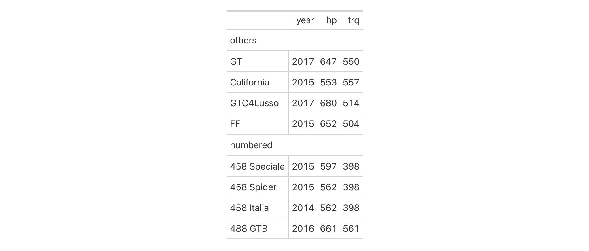
The above use of the row_group.default_label in tab_options() gets the
job done and provides a default label. One drawback is that the default/NA
group doesn't have an ID, so it can't as easily be styled with tab_style();
however, row groups have indices and the index for the "others" group here
is 1.
gtcars |>
dplyr::select(model, year, hp, trq) |>
dplyr::slice(1:8) |>
gt(rowname_col = "model") |>
tab_row_group(
label = "numbered",
rows = matches("^[0-9]")
) |>
row_group_order(groups = c(NA, "numbered")) |>
tab_options(row_group.default_label = "others") |>
tab_style(
style = cell_fill(color = "bisque"),
locations = cells_row_groups(groups = 1)
) |>
tab_style(
style = cell_fill(color = "lightgreen"),
locations = cells_row_groups(groups = "numbered")
)
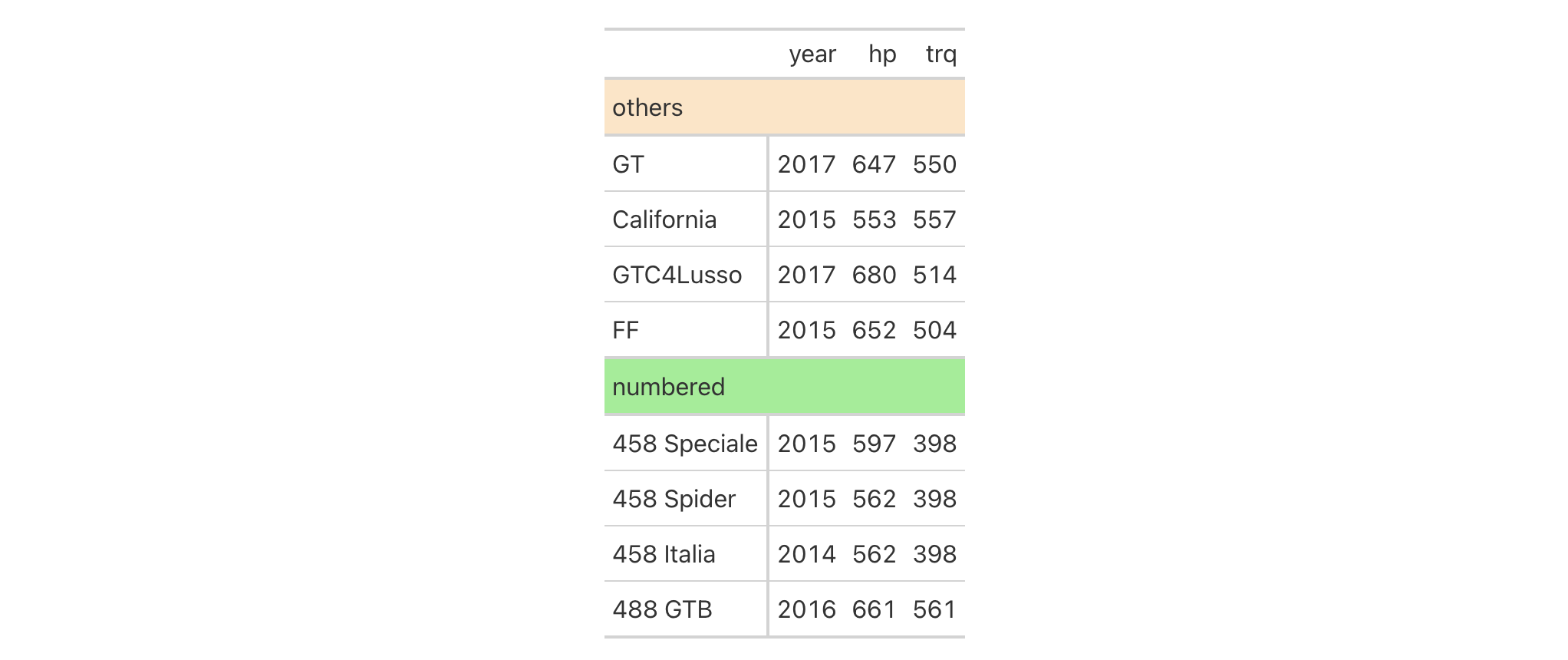
Now let's try using tab_row_group() with our gtcars-based table such
that all rows are formally assigned to different row groups. We'll define two
row groups with the (Markdown-infused) labels "**Powerful Cars**" and
"**Super Powerful Cars**". The distinction between the groups is whether
hp is lesser or greater than 600 (and this is governed by the expressions
provided to the rows argument).
gtcars |>
dplyr::select(model, year, hp, trq) |>
dplyr::slice(1:8) |>
gt(rowname_col = "model") |>
tab_row_group(
label = md("**Powerful Cars**"),
rows = hp < 600,
id = "powerful"
) |>
tab_row_group(
label = md("**Super Powerful Cars**"),
rows = hp >= 600,
id = "v_powerful"
) |>
tab_style(
style = cell_fill(color = "gray85"),
locations = cells_row_groups(groups = "powerful")
) |>
tab_style(
style = list(
cell_fill(color = "gray95"),
cell_text(size = "larger")
),
locations = cells_row_groups(groups = "v_powerful")
)
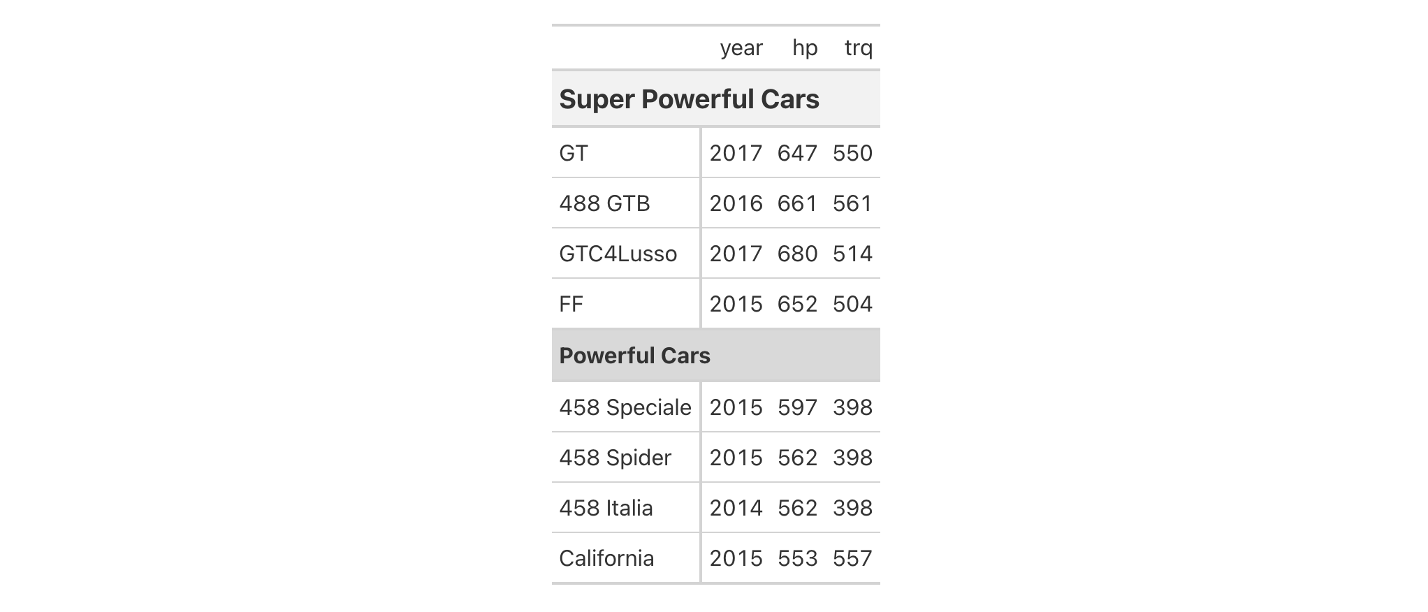
Setting the id values for each of the row groups makes things easier since
you will have clean, markup-free ID values to reference in later calls (as
was done with the tab_style() invocations in the example above). The use of
the md() helper function makes it so that any Markdown provided for the
label of a row group is faithfully rendered.
Function ID
2-4
Function Introduced
v0.2.0.5 (March 31, 2020)
See Also
Other part creation/modification functions:
tab_caption(),
tab_footnote(),
tab_header(),
tab_info(),
tab_options(),
tab_source_note(),
tab_spanner(),
tab_spanner_delim(),
tab_stub_indent(),
tab_stubhead(),
tab_style(),
tab_style_body()
Add a source note citation
Description
Add a source note to the footer part of the gt table. A source note is
useful for citing the data included in the table. Several can be added to the
footer, simply use multiple calls of tab_source_note() and they will be
inserted in the order provided. We can use Markdown formatting for the note,
or, if the table is intended for HTML output, we can include HTML formatting.
Usage
tab_source_note(data, source_note)tab_source_note(data, source_note)
Arguments
data |
The gt table data object
This is the gt table object that is commonly created through use of the
|
source_note |
Source note text
Text to be used in the source note. We can optionally use |
Value
An object of class gt_tbl.
Examples
With three columns from the gtcars dataset, let's create a gt table.
We can use tab_source_note() to add a source note to the table
footer. Here we are citing the data source but this function can be used for
any text you'd prefer to display in the footer section.
gtcars |> dplyr::select(mfr, model, msrp) |> dplyr::slice(1:5) |> gt() |> tab_source_note(source_note = "From edmunds.com")

Function ID
2-8
Function Introduced
v0.2.0.5 (March 31, 2020)
See Also
Other part creation/modification functions:
tab_caption(),
tab_footnote(),
tab_header(),
tab_info(),
tab_options(),
tab_row_group(),
tab_spanner(),
tab_spanner_delim(),
tab_stub_indent(),
tab_stubhead(),
tab_style(),
tab_style_body()
Add a spanner label
Description
With tab_spanner(), you can insert a spanner in the column labels part of a
gt table. This part of the table contains, at a minimum, column labels
and, optionally, an unlimited number of levels for spanners. A spanner will
occupy space over any number of contiguous column labels and it will have an
associated label and ID value. This function allows for mapping to be defined
by column names, existing spanner ID values, or a mixture of both. The
spanners are placed in the order of calling tab_spanner() so if a later call
uses the same columns in its definition (or even a subset) as the first
invocation, the second spanner will be overlaid atop the first. Options exist
for forcibly inserting a spanner underneath other (with level as space
permits) and with replace, which allows for full or partial spanner
replacement.
Usage
tab_spanner( data, label, columns = NULL, spanners = NULL, level = NULL, id = label, gather = TRUE, replace = FALSE )tab_spanner( data, label, columns = NULL, spanners = NULL, level = NULL, id = label, gather = TRUE, replace = FALSE )
Arguments
data |
The gt table data object
This is the gt table object that is commonly created through use of the
|
label |
Spanner label text
The text to use for the spanner label. We can optionally use |
columns |
Columns to target
The columns to serve as components of the spanner. Can either be a series
of column names provided in |
spanners |
Spanners to target
The spanners that should be spanned over, should they already be defined.
One or more spanner ID values (in quotes) can be supplied here. This
argument works in tandem with the |
level |
Spanner level for insertion
An explicit level to which the spanner should be placed. If not provided,
gt will choose the level based on the inputs provided within In combination with |
id |
Spanner ID
The ID for the spanner. When accessing a spanner through the |
gather |
Gather columns together
An option to move the specified |
replace |
Replace existing spanners
Should new spanners be allowed to partially or fully replace existing
spanners? (This is a possibility if setting spanners at an already
populated |
Value
An object of class gt_tbl.
Targeting columns with the columns argument
The columns argument allows us to target a subset of columns contained in
the table. We can declare column names in c() (with bare column names or
names in quotes) or we can use tidyselect-style expressions. This can be
as basic as supplying a select helper like starts_with(), or, providing a
more complex incantation like
where(~ is.numeric(.x) & max(.x, na.rm = TRUE) > 1E6)
which targets numeric columns that have a maximum value greater than
1,000,000 (excluding any NAs from consideration).
Details on spanner placement
Let's take a hypothetical table that includes the following column names in
order from left to right: year, len.pop, m.pop, len.dens, and
m.dens. We'd like to have some useful spanners, but don't want to have any
over the year column (so we'll avoid using that column when defining
spanners). Let's start by creating a schematic representation of what is
wanted in terms of spanners:
| ------- `"Two Provinces of Ireland"` ------ <- level 2 spanner
| ---- `"Leinster"` ---- | --- `"Munster"` -- <- level 1 spanners
`year` | `len.pop` | `len.dens` | `m.pop` | `m.dens` <- column names
----------------------------------------------------
To make this arrangement happen, we need three separate calls of
tab_spanner():
-
tab_spanner(., label = "Leinster", columns = starts_with("len")) -
tab_spanner(., label = "Munster", columns = starts_with("m")) -
tab_spanner(., label = "Two Provinces of Ireland", columns = -year)
This will give us the spanners we need with the appropriate labels. The ID
values will be derived from the labels in this case, but they can directly
supplied via the id argument.
An important thing to keep aware of is that the order of calls matters. The
first two can be in any order but the third one must happen last since we
build spanners from the bottom up. Also note that the first calls will
rearrange columns! This is by design as the gather = TRUE default will
purposefully gather columns together so that the columns will be united under
a single spanner. More complex definitions of spanners can be performed and
the Examples section demonstrates some of the more advanced calls of
tab_spanner().
As a final note, the column labels (by default deriving from the column
names) will likely need to change and that's especially true in the above
case. This can be done with either of cols_label() or cols_label_with().
Incorporating units with gt's units notation
Measurement units are often seen as part of spanner labels and indeed it can
be much more straightforward to include them here rather than using other
devices to make readers aware of units for specific columns. Any text
pertaining units is to be defined alongside the spanner label. To do this, we
have to surround the portion of text in the label that corresponds to the
units definition with "{{"/"}}".
Now that we know how to mark text for units definition, we know need to know how to write proper units with the notation. Such notation uses a succinct method of writing units and it should feel somewhat familiar though it is particular to the task at hand. Each unit is treated as a separate entity (parentheses and other symbols included) and the addition of subscript text and exponents is flexible and relatively easy to formulate. This is all best shown with a few examples:
-
"m/s"and"m / s"both render as"m/s" -
"m s^-1"will appear with the"-1"exponent intact -
"m /s"gives the same result, as"/<unit>"is equivalent to"<unit>^-1" -
"E_h"will render an"E"with the"h"subscript -
"t_i^2.5"provides atwith an"i"subscript and a"2.5"exponent -
"m[_0^2]"will use overstriking to set both scripts vertically -
"g/L %C6H12O6%"uses a chemical formula (enclosed in a pair of"%"characters) as a unit partial, and the formula will render correctly with subscripted numbers -
Common units that are difficult to write using ASCII text may be implicitly converted to the correct characters (e.g., the
"u"in"ug","um","uL", and"umol"will be converted to the Greek mu symbol;"degC"and"degF"will render a degree sign before the temperature unit) -
We can transform shorthand symbol/unit names enclosed in
":"(e.g.,":angstrom:",":ohm:", etc.) into proper symbols -
Greek letters can added by enclosing the letter name in
":"; you can use lowercase letters (e.g.,":beta:",":sigma:", etc.) and uppercase letters too (e.g.,":Alpha:",":Zeta:", etc.) -
The components of a unit (unit name, subscript, and exponent) can be fully or partially italicized/emboldened by surrounding text with
"*"or"**"
Examples
Let's create a gt table using a small portion of the gtcars dataset.
Over several columns (hp, hp_rpm, trq, trq_rpm, mpg_c, mpg_h)
we'll use tab_spanner() to add a spanner with the label "performance".
This effectively groups together several columns related to car performance
under a unifying label.
gtcars |>
dplyr::select(
-mfr, -trim, bdy_style,
-drivetrain, -trsmn, -ctry_origin
) |>
dplyr::slice(1:8) |>
gt(rowname_col = "model") |>
tab_spanner(
label = "performance",
columns = c(
hp, hp_rpm, trq, trq_rpm, mpg_c, mpg_h
)
)

With the default gather = TRUE option, columns selected for a particular
spanner will be moved so that there is no separation between them. This can
be seen with the example below that uses a subset of the towny dataset.
The starting column order is name, latitude, longitude,
population_2016, density_2016, population_2021, and density_2021. The
first two uses of tab_spanner() deal with making separate spanners for the
two population and two density columns. After their use, the columns are
moved to this new ordering: name, latitude, longitude,
population_2016, population_2021, density_2016, and density_2021. The
third and final call of tab_spanner() doesn't further affect the ordering
of columns.
towny |>
dplyr::slice_max(population_2021, n = 5) |>
dplyr::select(
name, latitude, longitude,
ends_with("2016"), ends_with("2021")
) |>
gt() |>
tab_spanner(
label = "Population",
columns = starts_with("pop")
) |>
tab_spanner(
label = "Density",
columns = starts_with("den")
) |>
tab_spanner(
label = md("*Location*"),
columns = ends_with("itude"),
id = "loc"
)

While columns are moved, it is only the minimal amount of moving required
(pulling in columns from the right) to ensure that columns are gathered under
the appropriate spanners. With the last call, there are two more things to
note: (1) label values can use the md() (or html()) helper functions to
help create styled text, and (2) an id value may be supplied for reference
later (e.g., for styling with tab_style() or applying footnotes with
tab_footnote()).
It's possible to stack multiple spanners atop each other with consecutive
calls of tab_spanner(). It's a bit like playing Tetris: putting a spanner
down anywhere there is another spanner (i.e., there are one or more shared
columns) means that second spanner will reside a level above the prior. Let's
look at a few examples to see how this works, and we'll also explore a few
lesser-known placement tricks. We'll use a cut down version of exibble
for this, set up a few level-1 spanners, and then place a level-2 spanner
over two other spanners.
exibble_narrow <- exibble |> dplyr::slice_head(n = 3)
exibble_narrow |>
gt() |>
tab_spanner(
label = "Row Information",
columns = c(row, group)
) |>
tab_spanner(
label = "Numeric Values",
columns = where(is.numeric),
id = "num_spanner"
) |>
tab_spanner(
label = "Text Values",
columns = c(char, fctr),
id = "text_spanner"
) |>
tab_spanner(
label = "Numbers and Text",
spanners = c("num_spanner", "text_spanner")
)

In the above example, we used the spanners argument to define where the
"Numbers and Text"-labeled spanner should reside. For that, we supplied the
"num_spanner" and "text_spanner" ID values for the two spanners
associated with the num, currency, char, and fctr columns.
Alternatively, we could have given those column names to the columns
argument and achieved the same result. You could actually use a combination
of spanners and columns to define where the spanner should be placed.
Here is an example of just that:
exibble_narrow_gt <-
exibble_narrow |>
gt() |>
tab_spanner(
label = "Numeric Values",
columns = where(is.numeric),
id = "num_spanner"
) |>
tab_spanner(
label = "Text Values",
columns = c(char, fctr),
id = "text_spanner"
) |>
tab_spanner(
label = "Text, Dates, Times, Datetimes",
columns = contains(c("date", "time")),
spanners = "text_spanner"
)
exibble_narrow_gt

And, again, we could have solely supplied all of the column names to
columns instead of using this hybrid approach, but it is interesting to
express the definition of spanners with this flexible combination.
What if you wanted to extend the above example and place a spanner above the
date, time, and datetime columns? If you tried that in the manner as
exemplified above, the spanner will be placed in the third level of spanners:
exibble_narrow_gt |>
tab_spanner(
label = "Date and Time Columns",
columns = contains(c("date", "time")),
id = "date_time_spanner"
)

Remember that the approach taken by tab_spanner() is to keep stacking atop
existing spanners. But, there is space next to the "Text Values" spanner on
the first level. You can either revise the order of tab_spanner() calls,
or, use the level argument to force the spanner into that level (so long
as there is space).
exibble_narrow_gt |>
tab_spanner(
label = "Date and Time Columns",
columns = contains(c("date", "time")),
level = 1,
id = "date_time_spanner"
)

That puts the spanner in the intended level. If there aren't free locations
available in the level specified you'll get an error stating which columns
cannot be used for the new spanner (this can be circumvented, if necessary,
with the replace = TRUE option). If you choose a level higher than the
maximum occupied, then the spanner will be dropped down. Again, these
behaviors are indicative of Tetris-like rules which tend to work well for the
application of spanners.
Using a subset of the towny dataset, we can create an interesting gt
table. First, only certain columns are selected from the dataset, some
filtering of rows is done, rows are sorted, and then only the first 10 rows
are kept. After the data is introduced to gt(), we then apply some spanner
labels using two calls of tab_spanner(). In the second of those, we
incorporate unit notation text (within "{{"/"}}") in the label to get a
display of nicely-formatted units.
towny |>
dplyr::select(
name, ends_with(c("2001", "2006")), matches("2001_2006")
) |>
dplyr::filter(population_2001 > 100000) |>
dplyr::slice_max(pop_change_2001_2006_pct, n = 10) |>
gt() |>
fmt_integer() |>
fmt_percent(columns = matches("change"), decimals = 1) |>
tab_spanner(
label = "Population",
columns = starts_with("pop")
) |>
tab_spanner(
label = "Density, {{*persons* km^-2}}",
columns = starts_with("density")
) |>
cols_label(
ends_with("01") ~ "2001",
ends_with("06") ~ "2006",
matches("change") ~ md("Population Change,<br>2001 to 2006")
) |>
cols_width(everything() ~ px(120))

Function ID
2-2
Function Introduced
v0.2.0.5 (March 31, 2020)
See Also
tab_spanner_delim() to create spanners and new column labels with
delimited column names.
Other part creation/modification functions:
tab_caption(),
tab_footnote(),
tab_header(),
tab_info(),
tab_options(),
tab_row_group(),
tab_source_note(),
tab_spanner_delim(),
tab_stub_indent(),
tab_stubhead(),
tab_style(),
tab_style_body()
Create column labels and spanners via delimited column names
Description
tab_spanner_delim() can take specially-crafted column names and generate
one or more spanners (and revise column labels at the same time). This is
done by splitting the column name by the specified delimiter text (delim)
and placing the fragments from top to bottom (i.e., higher-level spanners to
the column labels) or vice versa. Furthermore, neighboring text fragments on
different spanner levels that have the same text will be coalesced together.
For instance, having the three side-by-side column names rating_1,
rating_2, and rating_3 will (in the default case at least) result in a
spanner with the label "rating" above columns with the labels "1", "2",
and "3". There are many options in cols_spanner_delim() to slice and dice
delimited column names in different ways:
-
delimiter text: choose the delimiter text to use for the fragmentation of column names into spanners with the
delimargument -
direction and amount of splitting: we can choose to split n times according to a
limitargument, and, we get to specify from which side of the column name the splitting should commence -
reversal of fragments: we can reverse the order the fragments we get from the splitting procedure with the
reverseargument -
column constraints: it's possible to constrain which columns in a gt table should participate in spanner creation using vectors or tidyselect-style expressions
Usage
tab_spanner_delim( data, delim, columns = everything(), split = c("last", "first"), limit = NULL, reverse = FALSE )tab_spanner_delim( data, delim, columns = everything(), split = c("last", "first"), limit = NULL, reverse = FALSE )
Arguments
data |
The gt table data object
This is the gt table object that is commonly created through use of the
|
delim |
Delimiter for splitting
The delimiter text to use to split one of more column names (i.e., those
that are targeted via the |
columns |
Columns to target
The columns to consider for the splitting, relabeling, and spanner setting
operations. Can either be a series of column names provided in |
split |
Splitting side
Should the delimiter splitting occur from the |
limit |
Limit for splitting
An optional limit to place on the splitting procedure. The default |
reverse |
Reverse vector of split names
Should the order of split names be reversed? By default, this is |
Value
An object of class gt_tbl.
Details on column splitting
If we take a hypothetical table that includes the column names
province.NL_ZH.pop, province.NL_ZH.gdp, province.NL_NH.pop, and
province.NL_NH.gdp, we can see that we have a naming system that has a
well-defined structure. We start with the more general to the left
("province") and move to the more specific on the right ("pop"). If the
columns are in the table in this exact order, then things are in an ideal
state as the eventual spanner labels will form from this neighboring.
When using tab_spanner_delim() here with delim set as "." we get the
following text fragments:
-
province.NL_ZH.pop->"province","NL_ZH","pop" -
province.NL_ZH.gdp->"province","NL_ZH","gdp" -
province.NL_NH.pop->"province","NL_NH","pop" -
province.NL_NH.gdp->"province","NL_NH","gdp"
This gives us the following arrangement of column labels and spanner labels:
--------- `"province"` ---------- <- level 2 spanner ---`"NL_ZH"`--- | ---`"NL_NH"`--- <- level 1 spanners `"pop"`|`"gdp"` | `"pop"`|`"gdp"` <- column labels ---------------------------------
There might be situations where the same delimiter is used throughout but
only the last instance requires a splitting. With a pair of column names like
north_holland_pop and north_holland_area you would only want "pop" and
"area" to be column labels underneath a single spanner ("north_holland").
To achieve this, the split and limit arguments are used and the values
for each need to be split = "last" and limit = 1. This will give us
the following arrangement:
--`"north_holland"`-- <- level 1 spanner `"pop"` | `"area"` <- column labels ---------------------
Examples
With a subset of the towny dataset, we can create a gt table and then
use tab_spanner_delim() to automatically generate column spanner labels.
In this case we have some column names in the form population_<year>.
The underscore character is the delimiter that separates a common word
"population" and a year value. In this default way of splitting, fragments
to the right are lowest (really they become new column labels) and moving
left we get spanners. Let's have a look at how tab_spanner_delim() handles
these column names:
towny_subset_gt <-
towny |>
dplyr::select(name, starts_with("population")) |>
dplyr::filter(grepl("^F", name)) |>
gt() |>
tab_spanner_delim(delim = "_") |>
fmt_integer()
towny_subset_gt

The spanner created through this use of tab_spanner_delim() is
automatically given an ID value by gt. Because it's hard to know what the
ID value is, we can use tab_info() to inspect the table's indices and ID
values.
towny_subset_gt |> tab_info()

From this informational table, we see that the ID for the spanner is
"spanner-population_1996". Also, the columns are still accessible by the
original column names (tab_spanner_delim() did change their labels though).
Let's use tab_style() along with cells_column_spanners() to add some
styling to the spanner label of the towny_subset_gt table.
towny_subset_gt |>
tab_style(
style = cell_text(weight = "bold", transform = "capitalize"),
locations = cells_column_spanners(spanners = "spanner-population_1996")
)

We can plan ahead a bit and refashion the column names with dplyr before
introducing the table to gt() and tab_spanner_delim(). Here the column
labels have underscore delimiters where splitting is not wanted (so a period
or space character is used instead). The usage of tab_spanner_delim() gives
two levels of spanners. We can further touch up the labels after that with
cols_label_with() and text_transform().
towny |>
dplyr::slice_max(population_2021, n = 5) |>
dplyr::select(name, ends_with("pct")) |>
dplyr::rename_with(
.fn = function(x) {
x |>
sub("pop_change_", "Population Change.", x = _) |>
sub("_pct", ".pct", x = _)
}
) |>
gt(rowname_col = "name") |>
tab_spanner_delim(delim = ".") |>
fmt_number(decimals = 1, scale_by = 100) |>
cols_label_with(
fn = function(x) gsub("pct", "%", x)
) |>
text_transform(
fn = function(x) gsub("_", " - ", x, fixed = TRUE),
locations = cells_column_spanners()
) |>
tab_style(
style = cell_text(align = "center"),
locations = cells_column_labels()
) |>
tab_style(
style = "padding-right: 36px;",
locations = cells_body()
)

With a summarized, filtered, and pivoted version of the pizzaplace
dataset, we can create another gt table and then use
tab_spanner_delim() with the delimiter/separator also used in
tidyr::pivot_wider(). We can also process the generated column labels with
cols_label_with().
pizzaplace |>
dplyr::select(name, date, type, price) |>
dplyr::group_by(name, date, type) |>
dplyr::summarize(
revenue = sum(price),
sold = dplyr::n(),
.groups = "drop"
) |>
dplyr::filter(date %in% c("2015-01-01", "2015-01-02", "2015-01-03")) |>
dplyr::filter(type %in% c("classic", "veggie")) |>
tidyr::pivot_wider(
names_from = date,
names_sep = ".",
values_from = c(revenue, sold),
values_fn = sum,
names_sort = TRUE
) |>
gt(rowname_col = "name", groupname_col = "type") |>
tab_spanner_delim(delim = ".") |>
sub_missing(missing_text = "") |>
fmt_currency(columns = starts_with("revenue")) |>
data_color(
columns = starts_with("revenue"),
method = "numeric",
palette = c("white", "lightgreen")
) |>
cols_label_with(
fn = function(x) {
paste0(x, " (", vec_fmt_datetime(x, format = "E"), ")")
}
)

Function ID
2-3
Function Introduced
v0.2.0.5 (March 31, 2020)
See Also
tab_spanner() to manually create spanners with more control over
spanner labels.
Other part creation/modification functions:
tab_caption(),
tab_footnote(),
tab_header(),
tab_info(),
tab_options(),
tab_row_group(),
tab_source_note(),
tab_spanner(),
tab_stub_indent(),
tab_stubhead(),
tab_style(),
tab_style_body()
Control indentation of row labels in the stub
Description
Indentation of row labels is an effective way for establishing structure in a
table stub. tab_stub_indent() allows for fine control over row label
indentation in the stub. We can use an explicit definition of an indentation
level (with a number between 0 and 5), or, employ an indentation
directive using keywords ("increase"/"decrease").
Usage
tab_stub_indent(data, rows, indent = "increase")tab_stub_indent(data, rows, indent = "increase")
Arguments
data |
The gt table data object
This is the gt table object that is commonly created through use of the
|
rows |
Rows to target
The rows to consider for the indentation change. We can supply a vector of
row ID values within |
indent |
Indentation directive
An indentation directive either as a keyword describing the indentation
change or as an explicit integer value for directly setting the indentation
level. The keyword |
Value
An object of class gt_tbl.
Compatibility of arguments with the from_column() helper function
from_column() can be used with the indent argument of tab_stub_indent()
to obtain varying parameter values from a specified column within the table.
This means that each row label could be indented a little bit differently.
Please note that for this argument (indent), a from_column() call needs
to reference a column that has data of the numeric or integer type.
Additional columns for parameter values can be generated with cols_add()
(if not already present). Columns that contain parameter data can also be
hidden from final display with cols_hide().
Examples
Using a subset of the photolysis dataset within a gt table, we can
provide some indentation to all of the row labels in the stub via
tab_stub_indent(). Here we provide an indent value of 3 for a very
prominent indentation that clearly shows that the row labels are subordinate
to the two row group labels in this table ("inorganic reactions" and
"carbonyls").
photolysis |>
dplyr::select(cmpd_name, products, type, l, m, n) |>
dplyr::slice_head(n = 10) |>
gt(groupname_col = "type", rowname_col = "cmpd_name") |>
fmt_chem(columns = products) |>
fmt_scientific(columns = l) |>
tab_stub_indent(
rows = everything(),
indent = 3
)
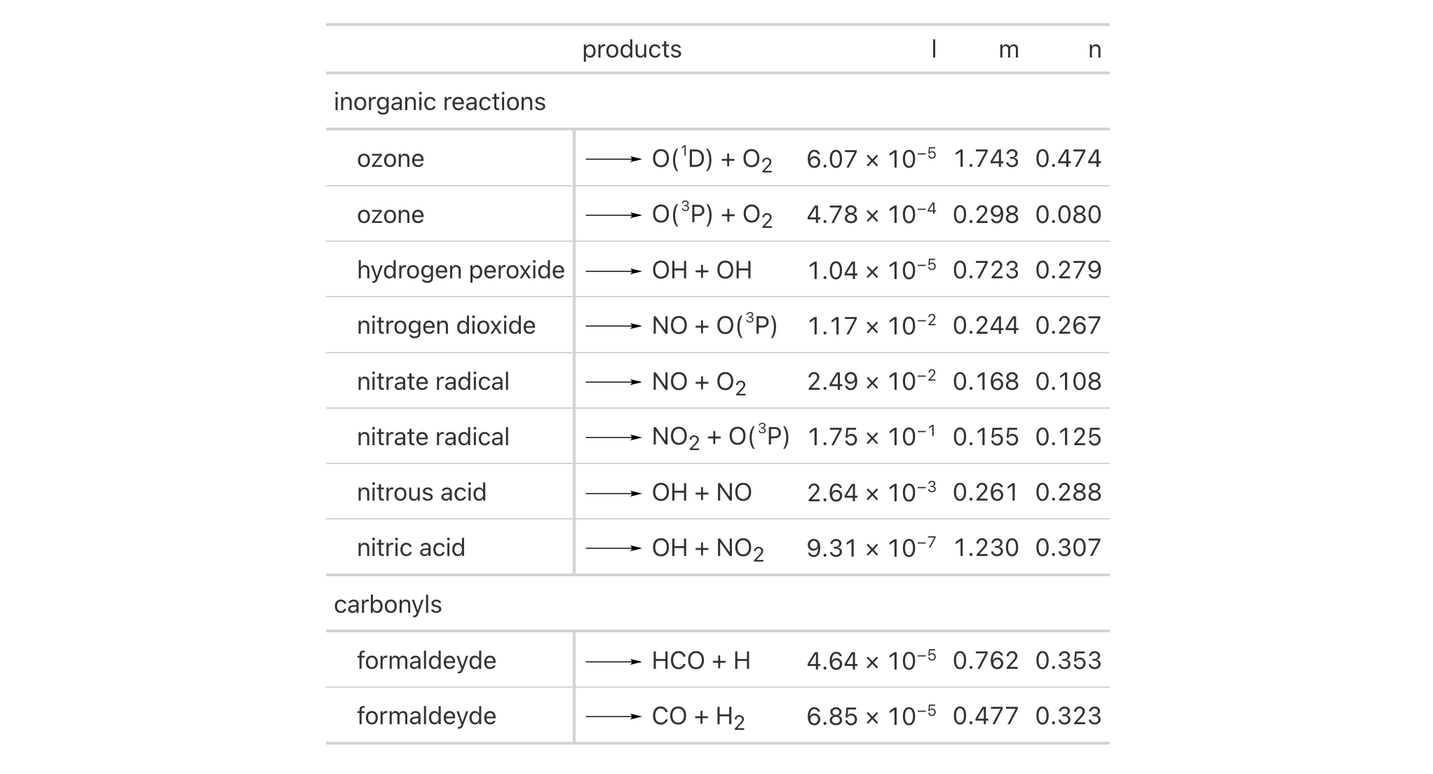
Let's use a summarized version of the pizzaplace dataset to create a
another gt table with row groups and row labels. With summary_rows(),
we'll generate summary rows at the top of each row group. Using
tab_stub_indent() we can add indentation to the row labels in the stub.
pizzaplace |>
dplyr::group_by(type, size) |>
dplyr::summarize(
sold = dplyr::n(),
income = sum(price),
.groups = "drop"
) |>
gt(rowname_col = "size", groupname_col = "type") |>
tab_header(title = "Pizzas Sold in 2015") |>
fmt_integer(columns = sold) |>
fmt_currency(columns = income) |>
summary_rows(
fns = list(label = "All Sizes", fn = "sum"),
side = "top",
fmt = list(
~ fmt_integer(., columns = sold),
~ fmt_currency(., columns = income)
)
) |>
tab_options(
summary_row.background.color = "gray95",
row_group.background.color = "#FFEFDB",
row_group.as_column = TRUE
) |>
tab_stub_indent(
rows = everything(),
indent = 2
)

Indentation of entries in the stub can be controlled by values within a
column. Here's an example of that using the constants dataset, where
variations of a row label are mutated to eliminate the common leading text
(replacing it with "..."). At the same time, the indentation for those rows
is set to 4 in the indent column (value is 0 otherwise). The
tab_stub_indent() statement uses from_column(), which passes values from
the indent column to the namesake argument. We hide the indent column
from view by use of cols_hide().
constants |>
dplyr::select(name, value, uncert, units) |>
dplyr::filter(
grepl("^atomic mass constant", name) |
grepl("^Rydberg constant", name) |
grepl("^Bohr magneton", name)
) |>
dplyr::mutate(
indent = ifelse(grepl("constant |magneton ", name), 4, 0),
name = gsub(".*constant |.*magneton ", "...", name)
) |>
gt(rowname_col = "name") |>
tab_stubhead(label = "Physical Constant") |>
tab_stub_indent(
rows = everything(),
indent = from_column(column = "indent")
) |>
fmt_scientific(columns = c(value, uncert)) |>
fmt_units(columns = units) |>
cols_hide(columns = indent) |>
cols_label(
value = "Value",
uncert = "Uncertainty",
units = "Units"
) |>
cols_width(
stub() ~ px(250),
c(value, uncert) ~ px(150),
units ~ px(80)
) |>
tab_style(
style = cell_text(indent = px(10)),
locations = list(
cells_column_labels(columns = units),
cells_body(columns = units)
)
)

Function ID
2-6
Function Introduced
v0.7.0 (Aug 25, 2022)
See Also
Other part creation/modification functions:
tab_caption(),
tab_footnote(),
tab_header(),
tab_info(),
tab_options(),
tab_row_group(),
tab_source_note(),
tab_spanner(),
tab_spanner_delim(),
tab_stubhead(),
tab_style(),
tab_style_body()
Add label text to the stubhead
Description
We can add a label to the stubhead of a gt table with tab_stubhead().
The stubhead is the lone part of the table that is positioned left of the
column labels, and above the stub. If a stub does not exist, then there is no
stubhead (so no visible change will be made when using this function in that
case). We have the flexibility to use Markdown formatting for the stubhead
label via the md() helper function. Furthermore, if the table is intended
for HTML output, we can use HTML inside of html() for the stubhead label.
Usage
tab_stubhead(data, label)tab_stubhead(data, label)
Arguments
data |
The gt table data object
This is the gt table object that is commonly created through use of the
|
label |
Stubhead label text
The text to be used as the stubhead label(s). For tables with multi-column
stubs, you can provide either a single label that spans all stub columns, or
a vector of labels with one label for each stub column. We can optionally use
|
Value
An object of class gt_tbl.
Examples
Using a small subset of the gtcars dataset, we can create a gt table
with row labels. Since we have row labels in the stub (via use of
rowname_col = "model" in the gt() function call) we have a stubhead, so,
let's add a stubhead label ("car") with tab_stubhead() to
describe what's in the stub.
gtcars |> dplyr::select(model, year, hp, trq) |> dplyr::slice(1:5) |> gt(rowname_col = "model") |> tab_stubhead(label = "car")

The stubhead can contain all sorts of interesting content. How about an icon for a car? We can make this happen with help from the fontawesome package.
gtcars |>
dplyr::select(model, year, hp, trq) |>
dplyr::slice(1:5) |>
gt(rowname_col = "model") |>
tab_stubhead(label = fontawesome::fa("car"))

If the stub is two columns wide (made possible by using
row_group_as_column = TRUE in the gt() statement), the stubhead will be a
merged cell atop those two stub columns representing the row group and the
row label. Here's an example of that type of situation in a table that uses
the peeps dataset.
peeps |>
dplyr::filter(country %in% c("POL", "DEU")) |>
dplyr::group_by(country) |>
dplyr::filter(dplyr::row_number() %in% 1:5) |>
dplyr::ungroup() |>
dplyr::mutate(name = paste0(toupper(name_family), ", ", name_given)) |>
dplyr::select(name, address, city, postcode, country) |>
gt(
rowname_col = "name",
groupname_col = "country",
row_group_as_column = TRUE
) |>
tab_stubhead(label = "Country Code / Person") |>
tab_style(
style = cell_text(transform = "capitalize"),
locations = cells_column_labels()
)

For tables with multi-column stubs (created by specifying multiple columns in
rowname_col), you can provide either a single label that spans all stub
columns, or a vector of labels with one label for each stub column. Here's an
example using the countrypops dataset with a single spanning label:
countrypops |>
dplyr::filter(country_name %in% c("China", "India", "United States", "Indonesia")) |>
dplyr::filter(year >= 2000) |>
dplyr::select(country_name, country_code_2, year, population) |>
gt(rowname_col = c("country_name", "country_code_2")) |>
tab_stubhead(label = "Country Information") |>
fmt_integer(columns = population)
Alternatively, you can provide a vector of labels, one for each stub column. This allows for more descriptive and specific headers for each column:
countrypops |>
dplyr::filter(country_name %in% c("China", "India", "United States", "Indonesia")) |>
dplyr::filter(year >= 2000) |>
dplyr::select(country_name, country_code_2, year, population) |>
gt(rowname_col = c("country_name", "country_code_2")) |>
tab_stubhead(label = c("Country", "Code")) |>
fmt_integer(columns = population)
You can also use this approach with three or more stub columns. Here's an example creating a hierarchical structure with region, country, and year:
countrypops |>
dplyr::filter(country_name %in% c("China", "India", "United States", "Indonesia")) |>
dplyr::filter(year %in% c(2000, 2010, 2020)) |>
dplyr::mutate(
region = dplyr::case_when(
country_name %in% c("China", "India", "Indonesia") ~ "Asia",
country_name == "United States" ~ "North America",
TRUE ~ "Other"
)
) |>
dplyr::select(region, country_name, year, population) |>
gt(rowname_col = c("region", "country_name", "year")) |>
tab_stubhead(label = c("Region", "Country", "Year")) |>
fmt_integer(columns = population)
Function ID
2-5
Function Introduced
v0.2.0.5 (March 31, 2020)
See Also
Other part creation/modification functions:
tab_caption(),
tab_footnote(),
tab_header(),
tab_info(),
tab_options(),
tab_row_group(),
tab_source_note(),
tab_spanner(),
tab_spanner_delim(),
tab_stub_indent(),
tab_style(),
tab_style_body()
Add custom styles to one or more cells
Description
With tab_style() we can target specific cells
and apply styles to them. This is best done in conjunction with the helper
functions cell_text(), cell_fill(), and cell_borders(). Currently, this
function is focused on the application of styles for HTML output only (as
such, other output formats will ignore all tab_style() calls). Using the
aforementioned helper functions, here are some of the styles we can apply:
-
the background color of the cell (
cell_fill():color) -
the cell's text color, font, and size (
cell_text():color,font,size) -
the text style (
cell_text():style), enabling the use of italics or oblique text. -
the text weight (
cell_text():weight), allowing the use of thin to bold text (the degree of choice is greater with variable fonts) -
the alignment and indentation of text (
cell_text():alignandindent) -
the cell borders (
cell_borders())
Usage
tab_style(data, style, locations)tab_style(data, style, locations)
Arguments
data |
The gt table data object
This is the gt table object that is commonly created through use of the
|
style |
Style declarations
The styles to use for the cells at the targeted |
locations |
Locations to target
The cell or set of cells to be associated with the style. Supplying any of
the |
Value
An object of class gt_tbl.
Using from_column() with cell_*() styling functions
from_column() can be used with certain arguments of cell_fill() and
cell_text(); this allows you to get parameter values from a specified
column within the table. This means that body cells targeted for styling
could be formatted a little bit differently, using options taken from a
column. For cell_fill(), we can use from_column() for its color
argument. cell_text() allows the use of from_column() in the following arguments:
-
color -
size -
align -
v_align -
style -
weight -
stretch -
decorate -
transform -
whitespace -
indent
Please note that for all of the aforementioned arguments, a from_column()
call needs to reference a column that has data of the correct type (this is
different for each argument). Additional columns for parameter values can be
generated with cols_add() (if not already present). Columns that contain
parameter data can also be hidden from final display with cols_hide().
Importantly, a tab_style() call with any use of from_column() within
styling expressions must only use cells_body() within locations. This is
because we cannot map multiple options taken from a column onto other
locations.
Examples
Let's use the exibble dataset to create a simple, two-column gt table
(keeping only the num and currency columns). With tab_style()
(called twice), we'll selectively add style to the values formatted by
fmt_number(). In the style argument of each tab_style() call, we can
define multiple types of styling with cell_fill() and cell_text()
(enclosed in a list). The cells to be targeted for styling require the use of
helpers like cells_body(), which is used here with different columns and
rows being targeted.
exibble |>
dplyr::select(num, currency) |>
gt() |>
fmt_number(decimals = 1) |>
tab_style(
style = list(
cell_fill(color = "lightcyan"),
cell_text(weight = "bold")
),
locations = cells_body(
columns = num,
rows = num >= 5000
)
) |>
tab_style(
style = list(
cell_fill(color = "#F9E3D6"),
cell_text(style = "italic")
),
locations = cells_body(
columns = currency,
rows = currency < 100
)
)

With a subset of the sp500 dataset, we'll create a different gt
table. Here, we'll color the background of entire rows of body cells and do
so on the basis of value expressions involving the open and close
columns.
sp500 |>
dplyr::filter(
date >= "2015-12-01" &
date <= "2015-12-15"
) |>
dplyr::select(-c(adj_close, volume)) |>
gt() |>
tab_style(
style = cell_fill(color = "lightgreen"),
locations = cells_body(rows = close > open)
) |>
tab_style(
style = list(
cell_fill(color = "red"),
cell_text(color = "white")
),
locations = cells_body(rows = open > close)
)
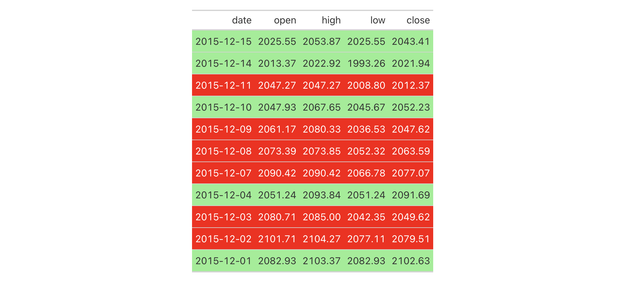
With another two-column table based on the exibble dataset, let's create
a gt table. First, we'll replace missing values with sub_missing().
Next, we'll add styling to the char column. This styling will be
HTML-specific and it will involve (all within a list): (1) a cell_fill()
call (to set a "lightcyan" background), and (2) a string containing a CSS
style declaration ("font-variant: small-caps;").
exibble |>
dplyr::select(char, fctr) |>
gt() |>
sub_missing() |>
tab_style(
style = list(
cell_fill(color = "lightcyan"),
"font-variant: small-caps;"
),
locations = cells_body(columns = char)
)

In the following table based on the towny dataset, we'll use a larger
number of tab_style() calls with the aim of styling each location available
in the table. Over six separate uses of tab_style(), different body cells
are styled with background colors, the header and the footer also receive
background color fills, borders are applied to a column of body cells and
also to the column labels, and, the row labels in the stub receive a custom
text treatment.
towny |>
dplyr::filter(csd_type == "city") |>
dplyr::select(
name, land_area_km2, density_2016, density_2021,
population_2016, population_2021
) |>
dplyr::slice_max(population_2021, n = 5) |>
gt(rowname_col = "name") |>
tab_header(
title = md(paste("Largest Five", fontawesome::fa("city") , "in `towny`")),
subtitle = "Changes in vital numbers from 2016 to 2021."
) |>
fmt_number(
columns = starts_with("population"),
n_sigfig = 3,
suffixing = TRUE
) |>
fmt_integer(columns = starts_with("density")) |>
fmt_number(columns = land_area_km2, decimals = 1) |>
cols_merge(
columns = starts_with("density"),
pattern = paste("{1}", fontawesome::fa("arrow-right"), "{2}")
) |>
cols_merge(
columns = starts_with("population"),
pattern = paste("{1}", fontawesome::fa("arrow-right"), "{2}")
) |>
cols_label(
land_area_km2 = md("Area, km^2^"),
starts_with("density") ~ md("Density, ppl/km^2^"),
starts_with("population") ~ "Population"
) |>
cols_align(align = "center", columns = -name) |>
cols_width(
stub() ~ px(125),
everything() ~ px(150)
) |>
tab_footnote(
footnote = "Data was used from their respective census-year publications.",
locations = cells_title(groups = "subtitle")
) |>
tab_source_note(source_note = md(
"All figures are compiled in the `towny` dataset (in the **gt** package)."
)) |>
opt_footnote_marks(marks = "letters") |>
tab_style(
style = list(
cell_fill(color = "gray95"),
cell_borders(sides = c("l", "r"), color = "gray50", weight = px(3))
),
locations = cells_body(columns = land_area_km2)
) |>
tab_style(
style = cell_fill(color = "lightblue" |> adjust_luminance(steps = 2)),
locations = cells_body(columns = -land_area_km2)
) |>
tab_style(
style = list(cell_fill(color = "gray35"), cell_text(color = "white")),
locations = list(cells_footnotes(), cells_source_notes())
) |>
tab_style(
style = cell_fill(color = "gray98"),
locations = cells_title()
) |>
tab_style(
style = cell_text(
size = "smaller",
weight = "bold",
transform = "uppercase"
),
locations = cells_stub()
) |>
tab_style(
style = cell_borders(
sides = c("t", "b"),
color = "powderblue",
weight = px(3)
),
locations = list(cells_column_labels(), cells_stubhead())
)
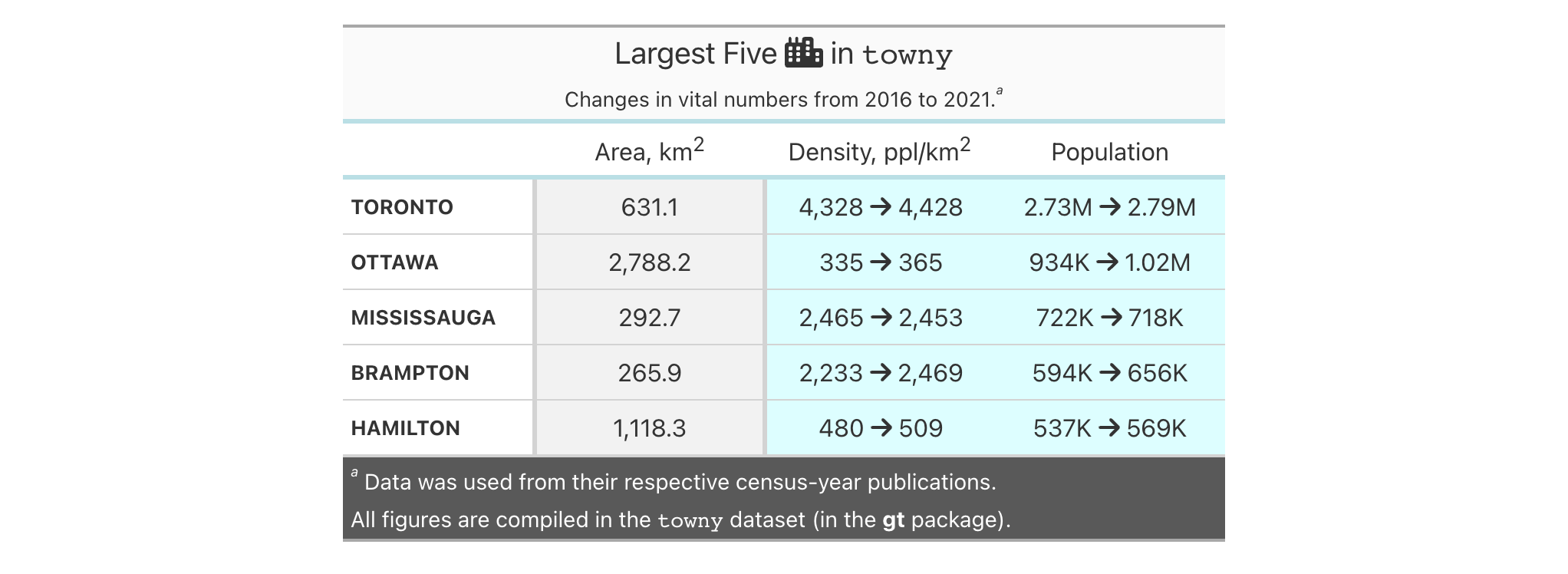
from_column() can be used to get values from a column. We'll use it in the
next example, which begins with a table having a color name column and a
column with the associated hexadecimal color code. To show the color in a
separate column, we first create one with cols_add() (ensuring that missing
values are replaced with "" via sub_missing()). Then, tab_style() is
used to style that column, using color = from_column()
within cell_fill().
dplyr::tibble(
name = c(
"red", "green", "blue", "yellow", "orange",
"cyan", "purple", "magenta", "lime", "pink"
),
hex = c(
"#E6194B", "#3CB44B", "#4363D8", "#FFE119", "#F58231",
"#42D4F4", "#911EB4", "#F032E6", "#BFEF45", "#FABED4"
)
) |>
gt(rowname_col = "name") |>
cols_add(color = rep(NA_character_, 10)) |>
sub_missing(missing_text = "") |>
tab_style(
style = cell_fill(color = from_column(column = "hex")),
locations = cells_body(columns = color)
) |>
tab_style(
style = cell_text(font = system_fonts(name = "monospace-code")),
locations = cells_body()
) |>
opt_all_caps() |>
cols_width(everything() ~ px(100)) |>
tab_options(table_body.hlines.style = "none")
cell_text() also allows the use of from_column() for many of its arguments.
Let's take a small portion of data from sp500 and add an up or down arrow
based on the values in the open and close columns. Within cols_add() we
can create a new column (dir) with an expression to get either "red" or
"green" text from a comparison of the open and close values. These
values are transformed to up or down arrows with text_case_match(), using
fontawesome icons in the end. However, the text values are still present
and can be used by cell_text() within tab_style(). from_column() makes
it possible to use the text in the cells of the dir column as color input
values.
sp500 |>
dplyr::filter(date > "2015-01-01") |>
dplyr::slice_min(date, n = 5) |>
dplyr::select(date, open, close) |>
gt(rowname_col = "date") |>
fmt_currency(columns = c(open, close)) |>
cols_add(dir = ifelse(close < open, "red", "forestgreen")) |>
cols_label(dir = "") |>
text_case_match(
"red" ~ fontawesome::fa("arrow-down"),
"forestgreen" ~ fontawesome::fa("arrow-up")
) |>
tab_style(
style = cell_text(color = from_column("dir")),
locations = cells_body(columns = dir)
)

Function ID
2-10
Function Introduced
v0.2.0.5 (March 31, 2020)
See Also
cell_text(), cell_fill(), and cell_borders() as helpers for
defining custom styles and cells_body() as one of many useful helper
functions for targeting the locations to be styled.
Other part creation/modification functions:
tab_caption(),
tab_footnote(),
tab_header(),
tab_info(),
tab_options(),
tab_row_group(),
tab_source_note(),
tab_spanner(),
tab_spanner_delim(),
tab_stub_indent(),
tab_stubhead(),
tab_style_body()
Target cells in the table body and style accordingly
Description
With tab_style_body() we can target cells through value, regex, and
custom matching rules and apply styles to them and their surrounding context
(i.e., styling an entire row or column wherein the match is found). Just as
with the general tab_style() function, this function is focused on the
application of styles for HTML output only (as such, other output formats
will ignore all tab_style() calls).
With the collection of cell_*() helper functions available in gt, we
can modify:
-
the background color of the cell (
cell_fill():color) -
the cell's text color, font, and size (
cell_text():color,font,size) -
the text style (
cell_text():style), enabling the use of italics or oblique text. -
the text weight (
cell_text():weight), allowing the use of thin to bold text (the degree of choice is greater with variable fonts) -
the alignment and indentation of text (
cell_text():alignandindent) -
the cell borders (
cell_borders())
Usage
tab_style_body( data, style, columns = everything(), rows = everything(), values = NULL, pattern = NULL, fn = NULL, targets = "cell", extents = "body" )tab_style_body( data, style, columns = everything(), rows = everything(), values = NULL, pattern = NULL, fn = NULL, targets = "cell", extents = "body" )
Arguments
data |
The gt table data object
This is the gt table object that is commonly created through use of the
|
style |
Style declarations
The styles to use for the targeted cells. |
columns |
Columns to target
The columns to which substitution operations are constrained. Can either
be a series of column names provided in |
rows |
Rows to target
In conjunction with |
values |
Values for targeting
The specific value or values that should be targeted for styling. If
|
pattern |
Regex pattern for targeting
A regex pattern that can target solely those values in |
fn |
Function to return logical values
A supplied function that operates on each cell of each column specified
through |
targets |
Styling targets
A vector of styling target keywords to contain or expand the target of each
cell. By default, this is a vector just containing |
extents |
Styling extents
A vector of locations to project styling. By default, this is a vector just
containing |
Value
An object of class gt_tbl.
Examples
Use exibble to create a gt table with a stub and row groups. This
contains an assortment of values that could potentially undergo some styling
via tab_style_body().
gt_tbl <-
exibble |>
gt(
rowname_col = "row",
groupname_col = "group"
)
Cells in the table body can be styled through specification of literal values
in the values argument of tab_style_body(). It's okay to search for
numerical, character, or logical values across all columns. Let's target the
values 49.95 and 33.33 and style those cells with an orange fill.
gt_tbl |>
tab_style_body(
style = cell_fill(color = "orange"),
values = c(49.95, 33.33)
)

Multiple styles can be combined in a list, here's an example of that using
the same cell targets:
gt_tbl |>
tab_style_body(
style = list(
cell_text(font = google_font("Inter"), color = "white"),
cell_fill(color = "red"),
cell_borders(
sides = c("left", "right"),
color = "steelblue",
weight = px(4)
)
),
values = c(49.95, 33.33)
)

You can opt to color entire rows or columns (or both, should you want to)
with those specific keywords in the targets argument. For the 49.95 value
we will style the entire row and with 33.33 the entire column will get the
same styling.
gt_tbl |>
tab_style_body(
style = cell_fill(color = "lightblue"),
values = 49.95,
targets = "row"
) |>
tab_style_body(
style = cell_fill(color = "lightblue"),
values = 33.33,
targets = "column"
)

In a minor variation to the prior example, it's possible to extend the
styling to other locations, or, entirely project the styling elsewhere. This
is done with the extents argument. Valid keywords that can be included in
the vector are: "body" (the default) and "stub". Let's take the previous
example and extend the styling of the row into the stub.
gt_tbl |>
tab_style_body(
style = cell_fill(color = "lightblue"),
values = 49.95,
targets = "row",
extents = c("body", "stub")
) |>
tab_style_body(
style = cell_fill(color = "lightblue"),
values = 33.33,
targets = "column"
)

We can also use the pattern argument to target cell values in
character-based columns. The "fctr" column is skipped because it is in
fact a factor-based column.
gt_tbl |>
tab_style_body(
style = cell_fill(color = "green"),
pattern = "ne|na"
)

For the most flexibility in targeting, it's best to use the fn argument.
The function you give to fn will be invoked separately on all cells so the
columns argument of tab_style_body() might be useful to limit which cells
should be evaluated. For this next example, the supplied function should only
be used on numeric values and we can make sure of this by using columns = where(is.numeric).
gt_tbl |>
tab_style_body(
columns = where(is.numeric),
style = cell_fill(color = "pink"),
fn = function(x) x >= 0 && x < 50
)

Styling every NA value in a table is also easily accomplished with the fn
argument by way of is.na().
gt_tbl |>
tab_style_body(
style = cell_text(color = "red3"),
fn = function(x) is.na(x)
) |>
sub_missing(missing_text = "Not Available")

Function ID
2-11
Function Introduced
v0.8.0 (November 16, 2022)
See Also
Other part creation/modification functions:
tab_caption(),
tab_footnote(),
tab_header(),
tab_info(),
tab_options(),
tab_row_group(),
tab_source_note(),
tab_spanner(),
tab_spanner_delim(),
tab_stub_indent(),
tab_stubhead(),
tab_style()
Generate a path to a test image
Description
Two test images are available within the gt package. Both contain the
same imagery (sized at 200px by 200px) but one is a PNG file while the other
is an SVG file. This function is most useful when paired with local_image()
since we test various sizes of the test image within that function.
Usage
test_image(type = c("png", "svg"))test_image(type = c("png", "svg"))
Arguments
type |
The image type
The type of image to produce here can either be |
Value
A character vector with a single path to an image file.
Function ID
9-4
Function Introduced
v0.2.0.5 (March 31, 2020)
See Also
Other image addition functions:
ggplot_image(),
local_image(),
web_image()
Perform whole or partial text replacements with a 'switch'-like approach
Description
text_case_match() provides a useful interface for a approach to replacing
table cells that behaves much like a switch statement. The targeting of cell
for transformation happens with the .locations argument. Once overall
targeting is handled, you need to supply a sequence of two-sided formulas
matching of the general form: <vector_old_text> ~ <new_text>. In the left
hand side (LHS) there should be a character vector containing strings to
match on. The right hand side (RHS) should contain a single string (or
something coercible to a length one character vector). There's also the
.replace argument that changes the matching and replacing behavior. By
default, text_case_match() will try to match on entire strings and replace
those strings. This can be changed to a partial matching and replacement
strategy with the alternate option.
Usage
text_case_match( .data, ..., .default = NULL, .replace = c("all", "partial"), .locations = cells_body() )text_case_match( .data, ..., .default = NULL, .replace = c("all", "partial"), .locations = cells_body() )
Arguments
.data |
The gt table data object
This is the gt table object that is commonly created through use of the
|
... |
Matching expressions
A sequence of two-sided formulas matching this general construction:
|
.default |
Default replacement text
The replacement text to use when cell values aren't matched by any of the
LHS inputs. If |
.replace |
Method for text replacement
A choice in how the matching is to be done. The default |
.locations |
Locations to target
The cell or set of cells to be associated with the text transformation.
Only |
Value
An object of class gt_tbl.
Examples
Let's use the exibble dataset to create a simple, two-column gt table
(keeping only the char and fctr columns). In the char column, we'll
transform the NA value to "elderberry" using the text_case_match()
function. Over in the fctr column, some more sophisticated matches will be
performed using text_case_match(). That column has spelled out numbers and
we can produce these on the LHS with help from vec_fmt_spelled_num().
The replacements will contain descriptive text. In this last call of
text_case_match(), we use a .default to replace text for any of those
non-matched cases.
exibble |>
dplyr::select(char, fctr) |>
gt() |>
text_case_match(
NA ~ "elderberry",
.locations = cells_body(columns = char)
) |>
text_case_match(
vec_fmt_spelled_num(1:4) ~ "one to four",
vec_fmt_spelled_num(5:6) ~ "five or six",
.default = "seven or more",
.locations = cells_body(columns = fctr)
)

Next, let's use a transformed version of the towny dataset to create a
gt table. Transform the text in the csd_type column using two-sided
formulas supplied to text_case_match(). We can replace matches on the LHS
with Fontawesome icons furnished by the fontawesome R package.
towny |>
dplyr::select(name, csd_type, population_2021) |>
dplyr::filter(csd_type %in% c("city", "town")) |>
dplyr::slice_max(population_2021, n = 5, by = csd_type) |>
dplyr::arrange(csd_type) |>
gt() |>
fmt_integer() |>
text_case_match(
"city" ~ fontawesome::fa("city"),
"town" ~ fontawesome::fa("house-chimney")
) |>
cols_label(
name = "City/Town",
csd_type = "",
population_2021 = "Population"
)

Function ID
4-3
Function Introduced
v0.9.0 (Mar 31, 2023)
See Also
Other text transforming functions:
text_case_when(),
text_replace(),
text_transform()
Perform whole text replacements using a 'case-when'-expression approach
Description
text_case_when() provides a useful interface for a case-by-case approach to
replacing entire table cells. First off, you have to make sure you're
targeting the appropriate cells with the .locations argument. Following
that, you supply a sequence of two-sided formulas matching of the general
form: <logical_stmt> ~ <new_text>. In the left hand side (LHS) there should
be a predicate statement that evaluates to a logical vector of length one
(i.e., either TRUE or FALSE). To refer to the values undergoing
transformation, you need to use the x variable.
Usage
text_case_when(.data, ..., .default = NULL, .locations = cells_body())text_case_when(.data, ..., .default = NULL, .locations = cells_body())
Arguments
.data |
The gt table data object
This is the gt table object that is commonly created through use of the
|
... |
Matching expressions
A sequence of two-sided formulas. The left hand side (LHS)
determines which values match this case. The right hand side (RHS) provides
the replacement text (it must resolve to a value of the |
.default |
Default replacement text
The replacement text to use when cell values aren't matched by any of the
LHS inputs. If |
.locations |
Locations to target
The cell or set of cells to be associated with the text transformation.
Only |
Value
An object of class gt_tbl.
Examples
Use a portion of the metro dataset to create a gt table. We'll use
text_case_when() to supply pairs of predicate statements and replacement
text. For the connect_rer column, we will perform a count of pattern
matches with stringr::str_count() and determine which cells have 1, 2, or 3
matched patterns. For each of these cases, descriptive replacement text is
provided. Here, we use a .default value to replace the non-matched
cases with an empty string (""). Finally, we use cols_label() to modify
the labels of the three columns.
metro |>
dplyr::slice_max(passengers, n = 10) |>
dplyr::select(name, lines, connect_rer) |>
gt() |>
text_case_when(
stringr::str_count(x, pattern = "[ABCDE]") == 1 ~ "One connection.",
stringr::str_count(x, pattern = "[ABCDE]") == 2 ~ "Two connections.",
stringr::str_count(x, pattern = "[ABCDE]") == 3 ~ "Three connections.",
.default = "", .locations = cells_body(columns = connect_rer)
) |>
cols_label(
name = "Station",
lines = "Lines Serviced",
connect_rer = "RER Connections"
)
Function ID
4-2
Function Introduced
v0.9.0 (Mar 31, 2023)
See Also
Other text transforming functions:
text_case_match(),
text_replace(),
text_transform()
Perform highly targeted text replacement with a regex pattern
Description
text_replace() provides a specialized interface for replacing text
fragments in table cells with literal text. You need to ensure that you're
targeting the appropriate cells with the locations argument. Once that is
done, the remaining two values to supply are the regex pattern (pattern)
and the replacement for all matched text (replacement).
Usage
text_replace(data, pattern, replacement, locations = cells_body())text_replace(data, pattern, replacement, locations = cells_body())
Arguments
data |
The gt table data object
This is the gt table object that is commonly created through use of the
|
pattern |
Regex pattern to match with
A regex pattern used to target text fragments in the cells resolved in locations. |
replacement |
Replacement text
The replacement text for any matched text fragments. |
locations |
Locations to target
The cell or set of cells to be associated with the text transformation.
Only |
Value
An object of class gt_tbl.
Examples
Use the metro dataset to create a gt table. With cols_merge(),
we'll merge the name and caption columns together but only if caption
doesn't have an NA value (the special pattern syntax of "{1}<<({2})>>"
takes care of this). This merged content is now part of the name column.
We'd like to modify this further wherever there is text in parentheses:
(1) make that text italicized, and (2) introduce a line break before the text
in parentheses. We can do this with text_replace(). The pattern value of
"\\((.*?)\\)" will match on text between parentheses, and the inner
"(.*?)" is a capture group. The replacement value of
"<br>(<em>\\1</em>)" puts the capture group text "\\1" within <em>
tags, wraps literal parentheses around it, and prepends a line break tag.
metro |>
dplyr::select(name, caption, lines) |>
dplyr::slice(110:120) |>
gt() |>
cols_merge(
columns = c(name, caption),
pattern = "{1}<< ({2})>>"
) |>
text_replace(
locations = cells_body(columns = name),
pattern = "\\((.*?)\\)",
replacement = "<br>(<em>\\1</em>)"
)
Function ID
4-1
Function Introduced
v0.9.0 (Mar 31, 2023)
See Also
Other text transforming functions:
text_case_match(),
text_case_when(),
text_transform()
Perform text transformations with a custom function
Description
Text transforming in gt is the act of modifying formatted strings in
targeted cells. text_transform() provides the most flexibility of all the
text_*() functions in their family of functions. With it, you target the
cells to undergo modification in the locations argument while also
supplying a function to the fn argument. The function given to fn should
ideally at the very least take x as an input (it stands for the character
vector that is essentially the targeted cells) and return a character vector
of the same length as the input. Using the construction function(x) { .. }
for the function is recommended.
Usage
text_transform(data, fn, locations = cells_body())text_transform(data, fn, locations = cells_body())
Arguments
data |
The gt table data object
This is the gt table object that is commonly created through use of the
|
fn |
Function for text transformation
The function to use for text transformation. It should include |
locations |
Locations to target
The cell or set of cells to be associated with the text transformation.
Only |
Value
An object of class gt_tbl.
Examples
Use a subset of the sp500 dataset to create a gt table. Transform the
text in the date column using a function supplied to text_transform()
(via the fn argument). Note that the x in the fn = function (x) part
consists entirely of ISO 8601 date strings (which are acceptable as input to
vec_fmt_date() and vec_fmt_datetime()).
sp500 |>
dplyr::slice_head(n = 10) |>
dplyr::select(date, open, close) |>
dplyr::arrange(-dplyr::row_number()) |>
gt() |>
fmt_currency() |>
text_transform(
fn = function(x) {
paste0(
"<strong>",
vec_fmt_date(x, date_style = "m_day_year"),
"</strong>",
"—W",
vec_fmt_datetime(x, format = "w")
)
},
locations = cells_body(columns = date)
) |>
cols_label(
date = "Date and Week",
open = "Opening Price",
close = "Closing Price"
)

Let's use a summarized version of the gtcars dataset to create a gt
table. First, the numeric values in the n column are formatted as
spelled-out numbers with fmt_spelled_num(). The output values are indeed
spelled out but exclusively with lowercase letters. We actually want these
words to begin with a capital letter and end with a period. To make this
possible, text_transform() will be used since it can modify
already-formatted text. Through the fn argument, we provide a custom
function that uses R's toTitleCase() operating on x (the numbers-as-text
strings) within paste0() so that a period can be properly placed.
gtcars |>
dplyr::filter(ctry_origin %in% c("Germany", "Italy", "Japan")) |>
dplyr::count(mfr, ctry_origin, sort = TRUE) |>
dplyr::arrange(ctry_origin) |>
gt(rowname_col = "mfr", groupname_col = "ctry_origin") |>
cols_label(n = "No. of Entries") |>
tab_stub_indent(rows = everything(), indent = 2) |>
cols_align(align = "center", columns = n) |>
fmt_spelled_num() |>
text_transform(
fn = function(x) {
paste0(tools::toTitleCase(x), ".")
},
locations = cells_body(columns = n)
)

There may be occasions where you'd want to remove all text. Here in this
example based on the pizzaplace dataset, we generate a gt table that
summarizes an entire year of data by colorizing the daily sales revenue.
Individual cell values are not needed here (since the encoding by color
suffices), so, text_transform() is used to turn every value to an empty
string: "".
pizzaplace |>
dplyr::group_by(date) |>
dplyr::summarize(rev = sum(price)) |>
dplyr::ungroup() |>
dplyr::mutate(
month = lubridate::month(date, label = TRUE),
day_num = lubridate::mday(date)
) |>
dplyr::select(-date) |>
tidyr::pivot_wider(names_from = month, values_from = rev) |>
gt(rowname_col = "day_num") |>
data_color(
method = "numeric",
palette = "wesanderson::Zissou1",
na_color = "white"
) |>
text_transform(
fn = function(x) "",
locations = cells_body()
) |>
opt_table_lines(extent = "none") |>
opt_all_caps() |>
cols_width(everything() ~ px(35)) |>
cols_align(align = "center")

Function ID
4-4
Function Introduced
v0.2.0.5 (March 31, 2020)
See Also
Other text transforming functions:
text_case_match(),
text_case_when(),
text_replace()
Populations of all municipalities in Ontario from 1996 to 2021
Description
A dataset containing census population data from six census years (1996 to 2021) for all 414 of Ontario's local municipalities. The Municipal Act of Ontario (2001) defines a local municipality as "a single-tier municipality or a lower-tier municipality". There are 173 single-tier municipalities and 241 lower-tier municipalities representing 99 percent of Ontario's population and 17 percent of its land use.
In the towny dataset we include information specific to each municipality
such as location (in the latitude and longitude columns), their website
URLs, their classifications, and land area sizes according to 2021
boundaries. Additionally, there are computed columns containing population
density values for each census year and population change values from
adjacent census years.
Usage
townytowny
Format
A tibble with 414 rows and 25 variables:
- name
-
The name of the municipality.
- website
-
The website for the municipality. This is
NAif there isn't an official site. - status
-
The status of the municipality. This is either
"lower-tier"or"single-tier". A single-tier municipality, which takes on all municipal duties outlined in the Municipal Act and other Provincial laws, is independent of an upper-tier municipality. Part of an upper-tier municipality is a lower-tier municipality. The upper-tier and lower-tier municipalities are responsible for carrying out the duties laid out in the Municipal Act and other provincial laws. - csd_type
-
The Census Subdivision Type. This can be one of
"village","town","township","municipality", or"city". - census_div
-
The Census division, of which there are 49. This is made up of single-tier municipalities, regional municipalities, counties, and districts.
- latitude, longitude
-
The location of the municipality, given as latitude and longitude values in decimal degrees.
- land_area_km2
-
The total area of the local municipality in square kilometers.
- population_1996, population_2001, population_2006, population_2011, population_2016, population_2021
-
Population values for each municipality from the 1996 to 2021 census years.
- density_1996, density_2001, density_2006, density_2011, density_2016, density_2021
-
Population density values, calculated as persons per square kilometer, for each municipality from the 1996 to 2021 census years.
- pop_change_1996_2001_pct, pop_change_2001_2006_pct, pop_change_2006_2011_pct, pop_change_2011_2016_pct, pop_change_2016_2021_pct
-
Population changes between adjacent pairs of census years, from 1996 to 2021.
Dataset ID and Badge
DATA-7

Dataset Introduced
v0.9.0 (Mar 31, 2023)
See Also
Other datasets:
constants,
countrypops,
exibble,
films,
gibraltar,
gtcars,
illness,
metro,
nuclides,
peeps,
photolysis,
pizzaplace,
reactions,
rx_addv,
rx_adsl,
sp500,
sza
Examples
dplyr::glimpse(towny)dplyr::glimpse(towny)
Get a conversion factor across two measurement units of a given class
Description
The unit_conversion() helper function gives us a conversion factor for
transforming a value from one form of measurement units to a target form.
For example if you have a length value that is expressed in miles you could
transform that value to one in kilometers through multiplication of the value
by the conversion factor (in this case 1.60934).
For unit_conversion() to understand the source and destination units, you
need to provide a keyword value for the from and to arguments. To aid as
a reference for this, call info_unit_conversions() to display an
information table that contains all of the keywords for every conversion
type.
Usage
unit_conversion(from, to)unit_conversion(from, to)
Arguments
from |
Units for the input value
The keyword representing the units for the value that requires unit
conversion. In the case where the value has units of miles, the necessary
input is |
to |
Desired units for the value
The keyword representing the target units for the value with units defined
in |
Value
A single numerical value.
Examples
Let's use a portion of the towny dataset and create a table showing
population, density, and land area for 10 municipalities. The land_area_km2
values are in units of square kilometers, however, we'd rather the values
were in square miles. We can convert the numeric values while formatting the
values with fmt_number() by using unit_conversion() in the scale_by
argument since the return value of that is a conversion factor (which is
applied to each value by multiplication). The same is done for converting the
'people per square kilometer' values in density_2021 to 'people per square
mile', however, the units to convert are in the denominator so the inverse
of the conversion factor must be used.
towny |>
dplyr::slice_max(density_2021, n = 10) |>
dplyr::select(name, population_2021, density_2021, land_area_km2) |>
gt(rowname_col = "name") |>
fmt_integer(columns = population_2021) |>
fmt_number(
columns = land_area_km2,
decimals = 1,
scale_by = unit_conversion(
from = "area.square-kilometer",
to = "area.square-mile"
)
) |>
fmt_number(
columns = density_2021,
decimals = 1,
scale_by = 1 / unit_conversion(
from = "area.square-kilometer",
to = "area.square-mile"
)
) |>
cols_label(
land_area_km2 = "Land Area,<br>sq. mi",
population_2021 = "Population",
density_2021 = "Density,<br>ppl / sq. mi",
.fn = md
)

With a small slice of the gibraltar dataset, let's display the
temperature values in terms of degrees Celsius (present in the data) and as
temperatures in degrees Fahrenheit (achievable via conversion). We can
duplicate the temp column through cols_add() (naming the new column as
temp_f) and when formatting through fmt_integer() we can call
unit_conversion() within the scale_by argument to perform this
transformation while formatting the values as integers.
gibraltar |>
dplyr::filter(
date == "2023-05-15",
time >= "06:00",
time <= "12:00"
) |>
dplyr::select(time, temp) |>
gt() |>
tab_header(
title = "Air Temperature During Late Morning Hours at LXGB Stn.",
subtitle = "May 15, 2023"
) |>
cols_add(temp_f = temp) |>
cols_move(columns = temp_f, after = temp) |>
tab_spanner(
label = "Temperature",
columns = starts_with("temp")
) |>
fmt_number(
columns = temp,
decimals = 1
) |>
fmt_integer(
columns = temp_f,
scale_by = unit_conversion(
from = "temperature.C",
to = "temperature.F"
)
) |>
cols_label(
time = "Time",
temp = "{{degC}}",
temp_f = "{{degF}}"
) |>
cols_width(
starts_with("temp") ~ px(80),
time ~ px(100)
) |>
opt_horizontal_padding(scale = 3) |>
opt_vertical_padding(scale = 0.5) |>
opt_align_table_header(align = "left") |>
tab_options(heading.title.font.size = px(16))

Function ID
8-7
Function Introduced
v0.11.0 (July 9, 2024)
See Also
Other helper functions:
adjust_luminance(),
cell_borders(),
cell_fill(),
cell_text(),
currency(),
default_fonts(),
escape_latex(),
from_column(),
google_font(),
gt_latex_dependencies(),
html(),
latex(),
md(),
nanoplot_options(),
pct(),
px(),
random_id(),
row_group(),
stub(),
system_fonts()
Format a vector as values in terms of bytes
Description
With numeric values in a vector, we can transform each into byte values with
human readable units. vec_fmt_bytes() allows for the formatting of byte
sizes to either of two common representations: (1) with decimal units
(powers of 1000, examples being "kB" and "MB"), and (2) with binary units
(powers of 1024, examples being "KiB" and "MiB").
It is assumed the input numeric values represent the number of bytes and automatic truncation of values will occur. The numeric values will be scaled to be in the range of 1 to <1000 and then decorated with the correct unit symbol according to the standard chosen. For more control over the formatting of byte sizes, we can use the following options:
-
decimals: choice of the number of decimal places, option to drop trailing zeros, and a choice of the decimal symbol
-
digit grouping separators: options to enable/disable digit separators and provide a choice of separator symbol
-
pattern: option to use a text pattern for decoration of the formatted values
-
locale-based formatting: providing a locale ID will result in number formatting specific to the chosen locale
Usage
vec_fmt_bytes( x, standard = c("decimal", "binary"), decimals = 1, n_sigfig = NULL, drop_trailing_zeros = TRUE, drop_trailing_dec_mark = TRUE, use_seps = TRUE, pattern = "{x}", sep_mark = ",", dec_mark = ".", force_sign = FALSE, min_sep_threshold = 1, incl_space = TRUE, locale = NULL, output = c("auto", "plain", "html", "latex", "rtf", "word") )vec_fmt_bytes( x, standard = c("decimal", "binary"), decimals = 1, n_sigfig = NULL, drop_trailing_zeros = TRUE, drop_trailing_dec_mark = TRUE, use_seps = TRUE, pattern = "{x}", sep_mark = ",", dec_mark = ".", force_sign = FALSE, min_sep_threshold = 1, incl_space = TRUE, locale = NULL, output = c("auto", "plain", "html", "latex", "rtf", "word") )
Arguments
x |
The input vector
This is the input vector that will undergo transformation to a character vector of the same length. Values within the vector will be formatted. |
standard |
Standard used to express byte sizes
The form of expressing large byte sizes is divided between: (1) decimal
units (powers of 1000; e.g., |
decimals |
Number of decimal places
This corresponds to the exact number of decimal places to use. A value
such as |
n_sigfig |
Number of significant figures
A option to format numbers to n significant figures. By default, this is
|
drop_trailing_zeros |
Drop any trailing zeros
A logical value that allows for removal of trailing zeros (those redundant zeros after the decimal mark). |
drop_trailing_dec_mark |
Drop the trailing decimal mark
A logical value that determines whether decimal marks should always appear
even if there are no decimal digits to display after formatting (e.g., |
use_seps |
Use digit group separators
An option to use digit group separators. The type of digit group separator
is set by |
pattern |
Specification of the formatting pattern
A formatting pattern that allows for decoration of the formatted value. The
formatted value is represented by the |
sep_mark |
Separator mark for digit grouping
The string to use as a separator between groups of digits. For example,
using |
dec_mark |
Decimal mark
The string to be used as the decimal mark. For example, using
|
force_sign |
Forcing the display of a positive sign
Should the positive sign be shown for positive numbers (effectively showing
a sign for all numbers except zero)? If so, use |
min_sep_threshold |
Minimum digit threshold for grouping separators
The minimum number of digits required in the integer part of a number for
grouping separators to be applied. This parameter determines when digit
grouping begins based on the magnitude of values. The value |
incl_space |
Include a space between the value and the units
An option for whether to include a space between the value and the units. The default is to use a space character for separation. |
locale |
Locale identifier
An optional locale identifier that can be used for formatting values
according to the locale's rules. Examples include |
output |
Output format
The output style of the resulting character vector. This can either be
|
Value
A character vector.
Examples
Let's create a numeric vector for the next few examples:
num_vals <- c(3.24294e14, 8, 1362902, -59027, NA)
Using vec_fmt_bytes() with the default options will create a character
vector with values in bytes. Any NA values remain as NA values. The
rendering context will be autodetected unless specified in the output
argument (here, it is of the "plain" output type).
vec_fmt_bytes(num_vals)
#> [1] "324.3 TB" "8 B" "1.4 MB" "-59 kB" "NA"
We can change the number of decimal places with the decimals option:
vec_fmt_bytes(num_vals, decimals = 2)
#> [1] "324.29 TB" "8 B" "1.36 MB" "-59.03 kB" "NA"
If we are formatting for a different locale, we could supply the locale ID and gt will handle any locale-specific formatting options:
vec_fmt_bytes(num_vals, locale = "fi")
#> [1] "324,3 TB" "8 B" "1,4 MB" "-59 kB" "NA"
Should you need to have positive and negative signs on each of the output
values, use force_sign = TRUE:
vec_fmt_bytes(num_vals, force_sign = TRUE)
#> [1] "+324.3 TB" "+8 B" "+1.4 MB" "-59 kB" "NA"
As a last example, one can wrap the values in a pattern with the pattern
argument. Note here that NA values won't have the pattern applied.
vec_fmt_bytes(num_vals, pattern = "[{x}]")
#> [1] "[324.3 TB]" "[8 B]" "[1.4 MB]" "[-59 kB]" "NA"
Function ID
15-13
Function Introduced
v0.7.0 (Aug 25, 2022)
See Also
The variant function intended for formatting gt table data:
fmt_bytes().
Other vector formatting functions:
vec_fmt_currency(),
vec_fmt_date(),
vec_fmt_datetime(),
vec_fmt_duration(),
vec_fmt_engineering(),
vec_fmt_fraction(),
vec_fmt_index(),
vec_fmt_integer(),
vec_fmt_markdown(),
vec_fmt_number(),
vec_fmt_number_si(),
vec_fmt_partsper(),
vec_fmt_percent(),
vec_fmt_roman(),
vec_fmt_scientific(),
vec_fmt_spelled_num(),
vec_fmt_time()
Format a vector as currency values
Description
With numeric values in a vector, we can perform currency-based formatting.
This function supports both automatic formatting with a three-letter or
numeric currency code. We can also specify a custom currency that is
formatted according to the output context with the currency() helper
function. We have fine control over the conversion from numeric values to
currency values, where we could take advantage of the following options:
-
the currency: providing a currency code or common currency name will procure the correct currency symbol and number of currency subunits; we could also use the
currency()helper function to specify a custom currency -
currency symbol placement: the currency symbol can be placed before or after the values
-
decimals/subunits: choice of the number of decimal places, and a choice of the decimal symbol, and an option on whether to include or exclude the currency subunits (decimal portion)
-
negative values: choice of a negative sign or parentheses for values less than zero
-
digit grouping separators: options to enable/disable digit separators and provide a choice of separator symbol
-
scaling: we can choose to scale targeted values by a multiplier value
-
large-number suffixing: larger figures (thousands, millions, etc.) can be autoscaled and decorated with the appropriate suffixes
-
pattern: option to use a text pattern for decoration of the formatted currency values
-
locale-based formatting: providing a locale ID will result in currency formatting specific to the chosen locale; it will also retrieve the locale's currency if none is explicitly given
We can call info_currencies() for a useful reference on all of the possible
inputs to the currency argument.
Usage
vec_fmt_currency( x, currency = NULL, use_subunits = TRUE, decimals = NULL, drop_trailing_dec_mark = TRUE, use_seps = TRUE, accounting = FALSE, scale_by = 1, suffixing = FALSE, pattern = "{x}", sep_mark = ",", dec_mark = ".", force_sign = FALSE, min_sep_threshold = 1, placement = "left", incl_space = FALSE, locale = NULL, output = c("auto", "plain", "html", "latex", "rtf", "word") )vec_fmt_currency( x, currency = NULL, use_subunits = TRUE, decimals = NULL, drop_trailing_dec_mark = TRUE, use_seps = TRUE, accounting = FALSE, scale_by = 1, suffixing = FALSE, pattern = "{x}", sep_mark = ",", dec_mark = ".", force_sign = FALSE, min_sep_threshold = 1, placement = "left", incl_space = FALSE, locale = NULL, output = c("auto", "plain", "html", "latex", "rtf", "word") )
Arguments
x |
The input vector
This is the input vector that will undergo transformation to a character vector of the same length. Values within the vector will be formatted. |
currency |
Currency to use
The currency to use for the numeric value. This input can be
supplied as a 3-letter currency code (e.g., We can also use the |
use_subunits |
Show or hide currency subunits
An option for whether the subunits portion of a currency value should be
displayed. For example, with an input value of |
decimals |
Number of decimal places
The |
drop_trailing_dec_mark |
Drop the trailing decimal mark
A logical value that determines whether decimal marks should always appear
even if there are no decimal digits to display after formatting. For
example, when |
use_seps |
Use digit group separators
An option to use digit group separators. The type of digit group separator
is set by |
accounting |
Use accounting style
An option to use accounting style for values. Normally, negative values will be shown with a minus sign but using accounting style will instead put any negative values in parentheses. |
scale_by |
Scale values by a fixed multiplier
All numeric values will be multiplied by the |
suffixing |
Specification for large-number suffixing
The We can alternatively provide a character vector that serves as a
specification for which symbols are to be used for each of the value ranges.
These preferred symbols will replace the defaults (e.g.,
Including Any use of If using |
pattern |
Specification of the formatting pattern
A formatting pattern that allows for decoration of the formatted value. The
formatted value is represented by the |
sep_mark |
Separator mark for digit grouping
The string to use as a separator between groups of digits. For example,
using |
dec_mark |
Decimal mark
The string to be used as the decimal mark. For example, using
|
force_sign |
Forcing the display of a positive sign
Should the positive sign be shown for positive values (effectively showing
a sign for all values except zero)? If so, use |
min_sep_threshold |
Minimum digit threshold for grouping separators
The minimum number of digits required in the integer part of a number for
grouping separators to be applied. This parameter determines when digit
grouping begins based on the magnitude of values. The value |
placement |
Currency symbol placement
The placement of the currency symbol. This can be either be |
incl_space |
Include a space between the value and the currency symbol
An option for whether to include a space between the value and the currency symbol. The default is to not introduce a space character. |
locale |
Locale identifier
An optional locale identifier that can be used for formatting values
according to the locale's rules. Examples include |
output |
Output format
The output style of the resulting character vector. This can either be
|
Value
A character vector.
Examples
Let's create a numeric vector for the next few examples:
num_vals <- c(5.2, 8.65, 0, -5.3, NA)
Using vec_fmt_currency() with the default options will create a character
vector where the numeric values have been transformed to U.S. Dollars
("USD"). Furthermore, the rendering context will be autodetected unless
specified in the output argument (here, it is of the "plain" output
type).
vec_fmt_currency(num_vals)
#> [1] "$5.20" "$8.65" "$0.00" "-$5.30" "NA"
We can supply a currency code to the currency argument. Let's use British
Pounds through currency = "GBP":
vec_fmt_currency(num_vals, currency = "GBP")
#> [1] "GBP5.20" "GBP8.65" "GBP0.00" "-GBP5.30" "NA"
If we are formatting for a different locale, we could supply the locale ID and let gt handle all locale-specific formatting options:
vec_fmt_currency(num_vals, locale = "fr")
#> [1] "EUR5,20" "EUR8,65" "EUR0,00" "-EUR5,30" "NA"
There are many options for formatting values. Perhaps you need to have
explicit positive and negative signs? Use force_sign = TRUE for that.
vec_fmt_currency(num_vals, force_sign = TRUE)
#> [1] "+$5.20" "+$8.65" "$0.00" "-$5.30" "NA"
As a last example, one can wrap the values in a pattern with the pattern
argument. Note here that NA values won't have the pattern applied.
vec_fmt_currency(num_vals, pattern = "`{x}`")
#> [1] "`$5.20`" "`$8.65`" "`$0.00`" "`-$5.30`" "NA"
Function ID
15-9
Function Introduced
v0.7.0 (Aug 25, 2022)
See Also
The variant function intended for formatting gt table data:
fmt_currency().
Other vector formatting functions:
vec_fmt_bytes(),
vec_fmt_date(),
vec_fmt_datetime(),
vec_fmt_duration(),
vec_fmt_engineering(),
vec_fmt_fraction(),
vec_fmt_index(),
vec_fmt_integer(),
vec_fmt_markdown(),
vec_fmt_number(),
vec_fmt_number_si(),
vec_fmt_partsper(),
vec_fmt_percent(),
vec_fmt_roman(),
vec_fmt_scientific(),
vec_fmt_spelled_num(),
vec_fmt_time()
Format a vector as date values
Description
Format vector values to date values using one of 41 preset date styles. Input
can be in the form of POSIXt (i.e., datetimes), the Date type, or
character (must be in the ISO 8601 form of YYYY-MM-DD HH:MM:SS or
YYYY-MM-DD).
Usage
vec_fmt_date( x, date_style = "iso", pattern = "{x}", locale = NULL, output = c("auto", "plain", "html", "latex", "rtf", "word") )vec_fmt_date( x, date_style = "iso", pattern = "{x}", locale = NULL, output = c("auto", "plain", "html", "latex", "rtf", "word") )
Arguments
x |
The input vector
This is the input vector that will undergo transformation to a character vector of the same length. Values within the vector will be formatted. |
date_style |
Predefined style for dates
The date style to use. By default this is the short name |
pattern |
Specification of the formatting pattern
A formatting pattern that allows for decoration of the formatted value. The
formatted value is represented by the |
locale |
Locale identifier
An optional locale identifier that can be used for formatting values
according to the locale's rules. Examples include |
output |
Output format
The output style of the resulting character vector. This can either be
|
Value
A character vector.
Formatting with the date_style argument
We need to supply a preset date style to the date_style argument. The date
styles are numerous and can handle localization to any supported locale. A
large segment of date styles are termed flexible date formats and this means
that their output will adapt to any locale provided. That feature makes the
flexible date formats a better option for locales other than "en" (the
default locale).
The following table provides a listing of all date styles and their output
values (corresponding to an input date of 2000-02-29).
| Date Style | Output | Notes | |
| 1 | "iso" |
"2000-02-29" |
ISO 8601 |
| 2 | "wday_month_day_year" |
"Tuesday, February 29, 2000" |
|
| 3 | "wd_m_day_year" |
"Tue, Feb 29, 2000" |
|
| 4 | "wday_day_month_year" |
"Tuesday 29 February 2000" |
|
| 5 | "month_day_year" |
"February 29, 2000" |
|
| 6 | "m_day_year" |
"Feb 29, 2000" |
|
| 7 | "day_m_year" |
"29 Feb 2000" |
|
| 8 | "day_month_year" |
"29 February 2000" |
|
| 9 | "day_month" |
"29 February" |
|
| 10 | "day_m" |
"29 Feb" |
|
| 11 | "year" |
"2000" |
|
| 12 | "month" |
"February" |
|
| 13 | "day" |
"29" |
|
| 14 | "year.mn.day" |
"2000/02/29" |
|
| 15 | "y.mn.day" |
"00/02/29" |
|
| 16 | "year_week" |
"2000-W09" |
|
| 17 | "year_quarter" |
"2000-Q1" |
|
| 18 | "yMd" |
"2/29/2000" |
flexible |
| 19 | "yMEd" |
"Tue, 2/29/2000" |
flexible |
| 20 | "yMMM" |
"Feb 2000" |
flexible |
| 21 | "yMMMM" |
"February 2000" |
flexible |
| 22 | "yMMMd" |
"Feb 29, 2000" |
flexible |
| 23 | "yMMMEd" |
"Tue, Feb 29, 2000" |
flexible |
| 24 | "GyMd" |
"2/29/2000 A" |
flexible |
| 25 | "GyMMMd" |
"Feb 29, 2000 AD" |
flexible |
| 26 | "GyMMMEd" |
"Tue, Feb 29, 2000 AD" |
flexible |
| 27 | "yM" |
"2/2000" |
flexible |
| 28 | "Md" |
"2/29" |
flexible |
| 29 | "MEd" |
"Tue, 2/29" |
flexible |
| 30 | "MMMd" |
"Feb 29" |
flexible |
| 31 | "MMMEd" |
"Tue, Feb 29" |
flexible |
| 32 | "MMMMd" |
"February 29" |
flexible |
| 33 | "GyMMM" |
"Feb 2000 AD" |
flexible |
| 34 | "yQQQ" |
"Q1 2000" |
flexible |
| 35 | "yQQQQ" |
"1st quarter 2000" |
flexible |
| 36 | "Gy" |
"2000 AD" |
flexible |
| 37 | "y" |
"2000" |
flexible |
| 38 | "M" |
"2" |
flexible |
| 39 | "MMM" |
"Feb" |
flexible |
| 40 | "d" |
"29" |
flexible |
| 41 | "Ed" |
"29 Tue" |
flexible |
We can call info_date_style() in the console to view a similar table
of date styles with example output.
Examples
Let's create a character vector of dates in the ISO-8601 format for the next few examples:
str_vals <- c("2022-06-13", "2019-01-25", "2015-03-23", NA)
Using vec_fmt_date() (here with the "wday_month_day_year" date style)
will result in a character vector of formatted dates. Any NA values remain
as NA values. The rendering context will be autodetected unless specified
in the output argument (here, it is of the "plain" output type).
vec_fmt_date(str_vals, date_style = "wday_month_day_year")
#> [1] "Monday, June 13, 2022" "Friday, January 25, 2019" #> [3] "Monday, March 23, 2015" NA
We can choose from any of 41 different date formatting styles. Many of these
styles are flexible, meaning that the structure of the format will adapt
to different locales. Let's use the "yMMMEd" date style to demonstrate this
(first in the default locale of "en"):
vec_fmt_date(str_vals, date_style = "yMMMEd")
#> [1] "Mon, Jun 13, 2022" "Fri, Jan 25, 2019" "Mon, Mar 23, 2015" NA
Let's perform the same type of formatting in the French ("fr") locale:
vec_fmt_date(str_vals, date_style = "yMMMEd", locale = "fr")
#> [1] "lun. 13 juin 2022" "ven. 25 janv. 2019" "lun. 23 mars 2015" NA
We can always use info_date_style() to call up an info table that serves as
a handy reference to all of the date_style options.
As a last example, one can wrap the date values in a pattern with the
pattern argument. Note here that NA values won't have the pattern
applied.
vec_fmt_date(str_vals, pattern = "Date: {x}")
#> [1] "Date: 2022-06-13" "Date: 2019-01-25" "Date: 2015-03-23" NA
Function ID
15-14
Function Introduced
v0.7.0 (Aug 25, 2022)
See Also
The variant function intended for formatting gt table data:
fmt_date().
Other vector formatting functions:
vec_fmt_bytes(),
vec_fmt_currency(),
vec_fmt_datetime(),
vec_fmt_duration(),
vec_fmt_engineering(),
vec_fmt_fraction(),
vec_fmt_index(),
vec_fmt_integer(),
vec_fmt_markdown(),
vec_fmt_number(),
vec_fmt_number_si(),
vec_fmt_partsper(),
vec_fmt_percent(),
vec_fmt_roman(),
vec_fmt_scientific(),
vec_fmt_spelled_num(),
vec_fmt_time()
Format a vector as datetime values
Description
Format values in a vector to datetime values using either presets for the
date and time components or a formatting directive (this can either use a
CLDR datetime pattern or strptime formatting). Input can be in the form
of POSIXct (i.e., datetimes), the Date type, or character (must be in
the ISO 8601 form of YYYY-MM-DD HH:MM:SS or YYYY-MM-DD).
Usage
vec_fmt_datetime( x, date_style = "iso", time_style = "iso", sep = " ", format = NULL, tz = NULL, pattern = "{x}", locale = NULL, output = c("auto", "plain", "html", "latex", "rtf", "word") )vec_fmt_datetime( x, date_style = "iso", time_style = "iso", sep = " ", format = NULL, tz = NULL, pattern = "{x}", locale = NULL, output = c("auto", "plain", "html", "latex", "rtf", "word") )
Arguments
x |
The input vector
This is the input vector that will undergo transformation to a character vector of the same length. Values within the vector will be formatted. |
date_style |
Predefined style for dates
The date style to use. By default this is the short name |
time_style |
Predefined style for times
The time style to use. By default this is the short name |
sep |
Separator between date and time components
The separator string to use between the date and time components. By
default, this is a single space character ( |
format |
Date/time formatting string
An optional formatting string used for generating custom dates/times. If
used then the arguments governing preset styles ( |
tz |
Time zone
The time zone for printing dates/times (i.e., the output). The
default of |
pattern |
Specification of the formatting pattern
A formatting pattern that allows for decoration of the formatted value. The
formatted value is represented by the |
locale |
Locale identifier
An optional locale identifier that can be used for formatting values
according to the locale's rules. Examples include |
output |
Output format
The output style of the resulting character vector. This can either be
|
Value
A character vector.
Formatting with the date_style argument
We can supply a preset date style to the date_style argument to separately
handle the date portion of the output. The date styles are numerous and can
handle localization to any supported locale. A large segment of date styles
are termed flexible date formats and this means that their output will adapt
to any locale provided. That feature makes the flexible date formats a
better option for locales other than "en" (the default locale).
The following table provides a listing of all date styles and their output
values (corresponding to an input date of 2000-02-29).
| Date Style | Output | Notes | |
| 1 | "iso" |
"2000-02-29" |
ISO 8601 |
| 2 | "wday_month_day_year" |
"Tuesday, February 29, 2000" |
|
| 3 | "wd_m_day_year" |
"Tue, Feb 29, 2000" |
|
| 4 | "wday_day_month_year" |
"Tuesday 29 February 2000" |
|
| 5 | "month_day_year" |
"February 29, 2000" |
|
| 6 | "m_day_year" |
"Feb 29, 2000" |
|
| 7 | "day_m_year" |
"29 Feb 2000" |
|
| 8 | "day_month_year" |
"29 February 2000" |
|
| 9 | "day_month" |
"29 February" |
|
| 10 | "day_m" |
"29 Feb" |
|
| 11 | "year" |
"2000" |
|
| 12 | "month" |
"February" |
|
| 13 | "day" |
"29" |
|
| 14 | "year.mn.day" |
"2000/02/29" |
|
| 15 | "y.mn.day" |
"00/02/29" |
|
| 16 | "year_week" |
"2000-W09" |
|
| 17 | "year_quarter" |
"2000-Q1" |
|
| 18 | "yMd" |
"2/29/2000" |
flexible |
| 19 | "yMEd" |
"Tue, 2/29/2000" |
flexible |
| 20 | "yMMM" |
"Feb 2000" |
flexible |
| 21 | "yMMMM" |
"February 2000" |
flexible |
| 22 | "yMMMd" |
"Feb 29, 2000" |
flexible |
| 23 | "yMMMEd" |
"Tue, Feb 29, 2000" |
flexible |
| 24 | "GyMd" |
"2/29/2000 A" |
flexible |
| 25 | "GyMMMd" |
"Feb 29, 2000 AD" |
flexible |
| 26 | "GyMMMEd" |
"Tue, Feb 29, 2000 AD" |
flexible |
| 27 | "yM" |
"2/2000" |
flexible |
| 28 | "Md" |
"2/29" |
flexible |
| 29 | "MEd" |
"Tue, 2/29" |
flexible |
| 30 | "MMMd" |
"Feb 29" |
flexible |
| 31 | "MMMEd" |
"Tue, Feb 29" |
flexible |
| 32 | "MMMMd" |
"February 29" |
flexible |
| 33 | "GyMMM" |
"Feb 2000 AD" |
flexible |
| 34 | "yQQQ" |
"Q1 2000" |
flexible |
| 35 | "yQQQQ" |
"1st quarter 2000" |
flexible |
| 36 | "Gy" |
"2000 AD" |
flexible |
| 37 | "y" |
"2000" |
flexible |
| 38 | "M" |
"2" |
flexible |
| 39 | "MMM" |
"Feb" |
flexible |
| 40 | "d" |
"29" |
flexible |
| 41 | "Ed" |
"29 Tue" |
flexible |
We can call info_date_style() in the console to view a similar table of
date styles with example output.
Formatting with the time_style argument
We can supply a preset time style to the time_style argument to separately
handle the time portion of the output. There are many time styles and all of
them can handle localization to any supported locale. Many of the time styles
are termed flexible time formats and this means that their output will adapt
to any locale provided. That feature makes the flexible time formats a
better option for locales other than "en" (the default locale).
The following table provides a listing of all time styles and their output
values (corresponding to an input time of 14:35:00). It is noted which of
these represent 12- or 24-hour time. Some of the flexible formats (those
that begin with "E") include the day of the week. Keep this in mind
when pairing such time_style values with a date_style so as to avoid
redundant or repeating information.
| Time Style | Output | Notes | |
| 1 | "iso" |
"14:35:00" |
ISO 8601, 24h |
| 2 | "iso-short" |
"14:35" |
ISO 8601, 24h |
| 3 | "h_m_s_p" |
"2:35:00 PM" |
12h |
| 4 | "h_m_p" |
"2:35 PM" |
12h |
| 5 | "h_p" |
"2 PM" |
12h |
| 6 | "Hms" |
"14:35:00" |
flexible, 24h |
| 7 | "Hm" |
"14:35" |
flexible, 24h |
| 8 | "H" |
"14" |
flexible, 24h |
| 9 | "EHm" |
"Thu 14:35" |
flexible, 24h |
| 10 | "EHms" |
"Thu 14:35:00" |
flexible, 24h |
| 11 | "Hmsv" |
"14:35:00 GMT+00:00" |
flexible, 24h |
| 12 | "Hmv" |
"14:35 GMT+00:00" |
flexible, 24h |
| 13 | "hms" |
"2:35:00 PM" |
flexible, 12h |
| 14 | "hm" |
"2:35 PM" |
flexible, 12h |
| 15 | "h" |
"2 PM" |
flexible, 12h |
| 16 | "Ehm" |
"Thu 2:35 PM" |
flexible, 12h |
| 17 | "Ehms" |
"Thu 2:35:00 PM" |
flexible, 12h |
| 18 | "EBhms" |
"Thu 2:35:00 in the afternoon" |
flexible, 12h |
| 19 | "Bhms" |
"2:35:00 in the afternoon" |
flexible, 12h |
| 20 | "EBhm" |
"Thu 2:35 in the afternoon" |
flexible, 12h |
| 21 | "Bhm" |
"2:35 in the afternoon" |
flexible, 12h |
| 22 | "Bh" |
"2 in the afternoon" |
flexible, 12h |
| 23 | "hmsv" |
"2:35:00 PM GMT+00:00" |
flexible, 12h |
| 24 | "hmv" |
"2:35 PM GMT+00:00" |
flexible, 12h |
| 25 | "ms" |
"35:00" |
flexible |
We can call info_time_style() in the console to view a similar table of
time styles with example output.
Formatting with a CLDR datetime pattern
We can use a CLDR datetime pattern with the format argument to create
a highly customized and locale-aware output. This is a character string that
consists of two types of elements:
-
Pattern fields, which repeat a specific pattern character one or more times. These fields are replaced with date and time data when formatting. The character sets of
A-Zanda-zare reserved for use as pattern characters. -
Literal text, which is output verbatim when formatting. This can include:
-
Any characters outside the reserved character sets, including spaces and punctuation.
-
Any text between single vertical quotes (e.g.,
'text'). -
Two adjacent single vertical quotes (”), which represent a literal single quote, either inside or outside quoted text.
-
The number of pattern fields is quite sizable so let's first look at how some
CLDR datetime patterns work. We'll use the datetime string
"2018-07-04T22:05:09.2358(America/Vancouver)" for all of the examples that
follow.
-
"mm/dd/y"->"05/04/2018" -
"EEEE, MMMM d, y"->"Wednesday, July 4, 2018" -
"MMM d E"->"Jul 4 Wed" -
"HH:mm"->"22:05" -
"h:mm a"->"10:05 PM" -
"EEEE, MMMM d, y 'at' h:mm a"->"Wednesday, July 4, 2018 at 10:05 PM"
Here are the individual pattern fields:
Year
Calendar Year
This yields the calendar year, which is always numeric. In most cases the
length of the "y" field specifies the minimum number of digits to display,
zero-padded as necessary. More digits will be displayed if needed to show the
full year. There is an exception: "yy" gives use just the two low-order
digits of the year, zero-padded as necessary. For most use cases, "y" or
"yy" should be good enough.
| Field Patterns | Output |
"y" |
"2018" |
"yy" |
"18" |
"yyy" to "yyyyyyyyy" |
"2018" to "000002018"
|
Year in the Week in Year Calendar
This is the year in 'Week of Year' based calendars in which the year
transition occurs on a week boundary. This may differ from calendar year
"y" near a year transition. This numeric year designation is used in
conjunction with pattern character "w" in the ISO year-week calendar as
defined by ISO 8601.
| Field Patterns | Output |
"Y" |
"2018" |
"YY" |
"18" |
"YYY" to "YYYYYYYYY" |
"2018" to "000002018"
|
Quarter
Quarter of the Year: formatting and standalone versions
The quarter names are identified numerically, starting at 1 and ending at
4. Quarter names may vary along two axes: the width and the context. The
context is either 'formatting' (taken as a default), which the form used
within a complete date format string, or, 'standalone', the form for date
elements used independently (such as in calendar headers). The standalone
form may be used in any other date format that shares the same form of the
name. Here, the formatting form for quarters of the year consists of some run
of "Q" values whereas the standalone form uses "q".
| Field Patterns | Output | Notes |
"Q"/"q" |
"3" |
Numeric, one digit |
"QQ"/"qq" |
"03" |
Numeric, two digits (zero padded) |
"QQQ"/"qqq" |
"Q3" |
Abbreviated |
"QQQQ"/"qqqq" |
"3rd quarter" |
Wide |
"QQQQQ"/"qqqqq" |
"3" |
Narrow |
Month
Month: formatting and standalone versions
The month names are identified numerically, starting at 1 and ending at
12. Month names may vary along two axes: the width and the context. The
context is either 'formatting' (taken as a default), which the form used
within a complete date format string, or, 'standalone', the form for date
elements used independently (such as in calendar headers). The standalone
form may be used in any other date format that shares the same form of the
name. Here, the formatting form for months consists of some run of "M"
values whereas the standalone form uses "L".
| Field Patterns | Output | Notes |
"M"/"L" |
"7" |
Numeric, minimum digits |
"MM"/"LL" |
"07" |
Numeric, two digits (zero padded) |
"MMM"/"LLL" |
"Jul" |
Abbreviated |
"MMMM"/"LLLL" |
"July" |
Wide |
"MMMMM"/"LLLLL" |
"J" |
Narrow |
Week
Week of Year
Values calculated for the week of year range from 1 to 53. Week 1 for a
year is the first week that contains at least the specified minimum number of
days from that year. Weeks between week 1 of one year and week 1 of the
following year are numbered sequentially from 2 to 52 or 53 (if
needed).
There are two available field lengths. Both will display the week of year
value but the "ww" width will always show two digits (where weeks 1 to
9 are zero padded).
| Field Patterns | Output | Notes |
"w" |
"27" |
Minimum digits |
"ww" |
"27" |
Two digits (zero padded) |
Week of Month
The week of a month can range from 1 to 5. The first day of every month
always begins at week 1 and with every transition into the beginning of a
week, the week of month value is incremented by 1.
| Field Pattern | Output |
"W" |
"1"
|
Day
Day of Month
The day of month value is always numeric and there are two available field
length choices in its formatting. Both will display the day of month value
but the "dd" formatting will always show two digits (where days 1 to 9
are zero padded).
| Field Patterns | Output | Notes |
"d" |
"4" |
Minimum digits |
"dd" |
"04" |
Two digits, zero padded |
Day of Year
The day of year value ranges from 1 (January 1) to either 365 or 366
(December 31), where the higher value of the range indicates that the year is
a leap year (29 days in February, instead of 28). The field length specifies
the minimum number of digits, with zero-padding as necessary.
| Field Patterns | Output | Notes |
"D" |
"185" |
|
"DD" |
"185" |
Zero padded to minimum width of 2 |
"DDD" |
"185" |
Zero padded to minimum width of 3 |
Day of Week in Month
The day of week in month returns a numerical value indicating the number of times a given weekday had occurred in the month (e.g., '2nd Monday in March'). This conveniently resolves to predicable case structure where ranges of day of the month values return predictable day of week in month values:
-
days
1-7->1 -
days
8-14->2 -
days
15-21->3 -
days
22-28->4 -
days
29-31->5
| Field Pattern | Output |
"F" |
"1"
|
Modified Julian Date
The modified version of the Julian date is obtained by subtracting 2,400,000.5 days from the Julian date (the number of days since January 1, 4713 BC). This essentially results in the number of days since midnight November 17, 1858. There is a half day offset (unlike the Julian date, the modified Julian date is referenced to midnight instead of noon).
| Field Patterns | Output |
"g" to "ggggggggg" |
"58303" -> "000058303"
|
Weekday
Day of Week Name
The name of the day of week is offered in four different widths.
| Field Patterns | Output | Notes |
"E", "EE", or "EEE" |
"Wed" |
Abbreviated |
"EEEE" |
"Wednesday" |
Wide |
"EEEEE" |
"W" |
Narrow |
"EEEEEE" |
"We" |
Short |
Periods
AM/PM Period of Day
This denotes before noon and after noon time periods. May be upper or lowercase depending on the locale and other options. The wide form may be the same as the short form if the 'real' long form (e.g. 'ante meridiem') is not customarily used. The narrow form must be unique, unlike some other fields.
| Field Patterns | Output | Notes |
"a", "aa", or "aaa" |
"PM" |
Abbreviated |
"aaaa" |
"PM" |
Wide |
"aaaaa" |
"p" |
Narrow |
AM/PM Period of Day Plus Noon and Midnight
Provide AM and PM as well as phrases for exactly noon and midnight. May be upper or lowercase depending on the locale and other options. If the locale doesn't have the notion of a unique 'noon' (i.e., 12:00), then the PM form may be substituted. A similar behavior can occur for 'midnight' (00:00) and the AM form. The narrow form must be unique, unlike some other fields.
(a) input_midnight: "2020-05-05T00:00:00"
(b) input_noon: "2020-05-05T12:00:00"
| Field Patterns | Output | Notes |
"b", "bb", or "bbb" |
(a) "midnight" |
Abbreviated |
(b) "noon" |
||
"bbbb" |
(a) "midnight" |
Wide |
(b) "noon" |
||
"bbbbb" |
(a) "mi" |
Narrow |
(b) "n" |
Flexible Day Periods
Flexible day periods denotes things like 'in the afternoon', 'in the evening', etc., and the flexibility comes from a locale's language and script. Each locale has an associated rule set that specifies when the day periods start and end for that locale.
(a) input_morning: "2020-05-05T00:08:30"
(b) input_afternoon: "2020-05-05T14:00:00"
| Field Patterns | Output | Notes |
"B", "BB", or "BBB" |
(a) "in the morning" |
Abbreviated |
(b) "in the afternoon" |
||
"BBBB" |
(a) "in the morning" |
Wide |
(b) "in the afternoon" |
||
"BBBBB" |
(a) "in the morning" |
Narrow |
(b) "in the afternoon" |
Hours, Minutes, and Seconds
Hour 0-23
Hours from 0 to 23 are for a standard 24-hour clock cycle (midnight plus
1 minute is 00:01) when using "HH" (which is the more common width that
indicates zero-padding to 2 digits).
Using "2015-08-01T08:35:09":
| Field Patterns | Output | Notes |
"H" |
"8" |
Numeric, minimum digits |
"HH" |
"08" |
Numeric, 2 digits (zero padded) |
Hour 1-12
Hours from 1 to 12 are for a standard 12-hour clock cycle (midnight plus
1 minute is 12:01) when using "hh" (which is the more common width that
indicates zero-padding to 2 digits).
Using "2015-08-01T08:35:09":
| Field Patterns | Output | Notes |
"h" |
"8" |
Numeric, minimum digits |
"hh" |
"08" |
Numeric, 2 digits (zero padded) |
Hour 1-24
Using hours from 1 to 24 is a less common way to express a 24-hour clock
cycle (midnight plus 1 minute is 24:01) when using "kk" (which is the
more common width that indicates zero-padding to 2 digits).
Using "2015-08-01T08:35:09":
| Field Patterns | Output | Notes |
"k" |
"9" |
Numeric, minimum digits |
"kk" |
"09" |
Numeric, 2 digits (zero padded) |
Hour 0-11
Using hours from 0 to 11 is a less common way to express a 12-hour clock
cycle (midnight plus 1 minute is 00:01) when using "KK" (which is the
more common width that indicates zero-padding to 2 digits).
Using "2015-08-01T08:35:09":
| Field Patterns | Output | Notes |
"K" |
"7" |
Numeric, minimum digits |
"KK" |
"07" |
Numeric, 2 digits (zero padded) |
Minute
The minute of the hour which can be any number from 0 to 59. Use "m" to
show the minimum number of digits, or "mm" to always show two digits
(zero-padding, if necessary).
| Field Patterns | Output | Notes |
"m" |
"5" |
Numeric, minimum digits |
"mm" |
"06" |
Numeric, 2 digits (zero padded) |
Seconds
The second of the minute which can be any number from 0 to 59. Use "s"
to show the minimum number of digits, or "ss" to always show two digits
(zero-padding, if necessary).
| Field Patterns | Output | Notes |
"s" |
"9" |
Numeric, minimum digits |
"ss" |
"09" |
Numeric, 2 digits (zero padded) |
Fractional Second
The fractional second truncates (like other time fields) to the width
requested (i.e., count of letters). So using pattern "SSSS" will display
four digits past the decimal (which, incidentally, needs to be added manually
to the pattern).
| Field Patterns | Output |
"S" to "SSSSSSSSS" |
"2" -> "235000000"
|
Milliseconds Elapsed in Day
There are 86,400,000 milliseconds in a day and the "A" pattern will provide
the whole number. The width can go up to nine digits with "AAAAAAAAA" and
these higher field widths will result in zero padding if necessary.
Using "2011-07-27T00:07:19.7223":
| Field Patterns | Output |
"A" to "AAAAAAAAA" |
"439722" -> "000439722"
|
Era
The Era Designator
This provides the era name for the given date. The Gregorian calendar has two eras: AD and BC. In the AD year numbering system, AD 1 is immediately preceded by 1 BC, with nothing in between them (there was no year zero).
| Field Patterns | Output | Notes |
"G", "GG", or "GGG" |
"AD" |
Abbreviated |
"GGGG" |
"Anno Domini" |
Wide |
"GGGGG" |
"A" |
Narrow |
Time Zones
TZ // Short and Long Specific non-Location Format
The short and long specific non-location formats for time zones are suggested
for displaying a time with a user friendly time zone name. Where the short
specific format is unavailable, it will fall back to the short localized GMT
format ("O"). Where the long specific format is unavailable, it will fall
back to the long localized GMT format ("OOOO").
| Field Patterns | Output | Notes |
"z", "zz", or "zzz" |
"PDT" |
Short Specific |
"zzzz" |
"Pacific Daylight Time" |
Long Specific |
TZ // Common UTC Offset Formats
The ISO8601 basic format with hours, minutes and optional seconds fields is
represented by "Z", "ZZ", or "ZZZ". The format is equivalent to RFC 822
zone format (when the optional seconds field is absent). This is equivalent
to the "xxxx" specifier. The field pattern "ZZZZ" represents the long
localized GMT format. This is equivalent to the "OOOO" specifier. Finally,
"ZZZZZ" pattern yields the ISO8601 extended format with hours, minutes and
optional seconds fields. The ISO8601 UTC indicator Z is used when local
time offset is 0. This is equivalent to the "XXXXX" specifier.
| Field Patterns | Output | Notes |
"Z", "ZZ", or "ZZZ" |
"-0700" |
ISO 8601 basic format |
"ZZZZ" |
"GMT-7:00" |
Long localized GMT format |
"ZZZZZ" |
"-07:00" |
ISO 8601 extended format |
TZ // Short and Long Localized GMT Formats
The localized GMT formats come in two widths "O" (which removes the minutes
field if it's 0) and "OOOO" (which always contains the minutes field).
The use of the GMT indicator changes according to the locale.
| Field Patterns | Output | Notes |
"O" |
"GMT-7" |
Short localized GMT format |
"OOOO" |
"GMT-07:00" |
Long localized GMT format |
TZ // Short and Long Generic non-Location Formats
The generic non-location formats are useful for displaying a recurring wall
time (e.g., events, meetings) or anywhere people do not want to be overly
specific. Where either of these is unavailable, there is a fallback to the
generic location format ("VVVV"), then the short localized GMT format as
the final fallback.
| Field Patterns | Output | Notes |
"v" |
"PT" |
Short generic non-location format |
"vvvv" |
"Pacific Time" |
Long generic non-location format |
TZ // Short Time Zone IDs and Exemplar City Formats
These formats provide variations of the time zone ID and often include the
exemplar city. The widest of these formats, "VVVV", is useful for
populating a choice list for time zones, because it supports 1-to-1 name/zone
ID mapping and is more uniform than other text formats.
| Field Patterns | Output | Notes |
"V" |
"cavan" |
Short time zone ID |
"VV" |
"America/Vancouver" |
Long time zone ID |
"VVV" |
"Vancouver" |
The tz exemplar city |
"VVVV" |
"Vancouver Time" |
Generic location format |
TZ // ISO 8601 Formats with Z for +0000
The "X"-"XXX" field patterns represent valid ISO 8601 patterns for time
zone offsets in datetimes. The final two widths, "XXXX" and "XXXXX" allow
for optional seconds fields. The seconds field is not supported by the ISO
8601 specification. For all of these, the ISO 8601 UTC indicator Z is used
when the local time offset is 0.
| Field Patterns | Output | Notes |
"X" |
"-07" |
ISO 8601 basic format (h, optional m) |
"XX" |
"-0700" |
ISO 8601 basic format (h & m) |
"XXX" |
"-07:00" |
ISO 8601 extended format (h & m) |
"XXXX" |
"-0700" |
ISO 8601 basic format (h & m, optional s) |
"XXXXX" |
"-07:00" |
ISO 8601 extended format (h & m, optional s) |
TZ // ISO 8601 Formats (no use of Z for +0000)
The "x"-"xxxxx" field patterns represent valid ISO 8601 patterns for time
zone offsets in datetimes. They are similar to the "X"-"XXXXX" field
patterns except that the ISO 8601 UTC indicator Z will not be used when
the local time offset is 0.
| Field Patterns | Output | Notes |
"x" |
"-07" |
ISO 8601 basic format (h, optional m) |
"xx" |
"-0700" |
ISO 8601 basic format (h & m) |
"xxx" |
"-07:00" |
ISO 8601 extended format (h & m) |
"xxxx" |
"-0700" |
ISO 8601 basic format (h & m, optional s) |
"xxxxx" |
"-07:00" |
ISO 8601 extended format (h & m, optional s) |
Formatting with a strptime format code
Performing custom date/time formatting with the format argument can also
occur with a strptime format code. This works by constructing a string of
individual format codes representing formatted date and time elements. These
are all indicated with a leading %, literal characters are interpreted as
any characters not starting with a % character.
First off, let's look at a few format code combinations that work well
together as a strptime format. This will give us an intuition on how these
generally work. We'll use the datetime "2015-06-08 23:05:37.48" for all of
the examples that follow.
-
"%m/%d/%Y"->"06/08/2015" -
"%A, %B %e, %Y"->"Monday, June 8, 2015" -
"%b %e %a"->"Jun 8 Mon" -
"%H:%M"->"23:05" -
"%I:%M %p"->"11:05 pm" -
"%A, %B %e, %Y at %I:%M %p"->"Monday, June 8, 2015 at 11:05 pm"
Here are the individual format codes for the date components:
-
"%a"->"Mon"(abbreviated day of week name) -
"%A"->"Monday"(full day of week name) -
"%w"->"1"(day of week number in0..6; Sunday is0) -
"%u"->"1"(day of week number in1..7; Monday is1, Sunday7) -
"%y"->"15"(abbreviated year, using the final two digits) -
"%Y"->"2015"(full year) -
"%b"->"Jun"(abbreviated month name) -
"%B"->"June"(full month name) -
"%m"->"06"(month number) -
"%d"->"08"(day number, zero-padded) -
"%e"->"8"(day number without zero padding) -
"%j"->"159"(day of the year, always zero-padded) -
"%W"->"23"(week number for the year, always zero-padded) -
"%V"->"24"(week number for the year, following the ISO 8601 standard) -
"%C"->"20"(the century number)
Here are the individual format codes for the time components:
-
"%H"->"23"(24h hour) -
"%I"->"11"(12h hour) -
"%M"->"05"(minute) -
"%S"->"37"(second) -
"%OS3"->"37.480"(seconds with decimals;3decimal places here) -
%p->"pm"(AM or PM indicator)
Here are some extra formats that you may find useful:
-
"%z"->"+0000"(signed time zone offset, here using UTC) -
"%F"->"2015-06-08"(the date in the ISO 8601 date format) -
"%%"->"%"(the literal "%" character, in case you need it)
Examples
Let's create a character vector of datetime values in the ISO-8601 format for the next few examples:
str_vals <- c("2022-06-13 18:36", "2019-01-25 01:08", NA)
Using vec_fmt_datetime() with different date_style and time_style
options (here, date_style = "yMMMEd" and time_style = "Hm") will result
in a character vector of formatted datetime values. Any NA values remain as
NA values. The rendering context will be autodetected unless specified in
the output argument (here, it is of the "plain" output type).
vec_fmt_datetime( str_vals, date_style = "yMMMEd", time_style = "Hm" )
#> [1] "Mon, Jun 13, 2022 18:36" "Fri, Jan 25, 2019 01:08" NA
We can choose from any of 41 different date styles and 25 time formatting
styles. Many of these styles are flexible, meaning that the structure of the
format will adapt to different locales. Let's use a combination of the
"yMMMd" and "hms" date and time styles to demonstrate this (first in the
default locale of "en"):
vec_fmt_datetime( str_vals, date_style = "yMMMd", time_style = "hms" )
#> [1] "Jun 13, 2022 6:36:00 PM" "Jan 25, 2019 1:08:00 AM" NA
Let's perform the same type of formatting in the Italian ("it") locale:
vec_fmt_datetime( str_vals, date_style = "yMMMd", time_style = "hms", locale = "it" )
#> [1] "13 giu 2022 6:36:00 PM" "25 gen 2019 1:08:00 AM" NA
We can always use info_date_style() or info_time_style() to call up info
tables that serve as handy references to all of the date_style and
time_style options.
It's possible to supply our own time formatting pattern within the format
argument. One way is with a CLDR pattern, which is locale-aware:
vec_fmt_datetime(str_vals, format = "EEEE, MMMM d, y, h:mm a")
#> [1] "Monday, June 13, 2022, 06:36 PM" #> [2] "Friday, January 25, 2019, 01:08 AM" #> [3] NA
By using the locale argument, this can be formatted as Dutch datetime
values:
vec_fmt_datetime( str_vals, format = "EEEE, MMMM d, y, h:mm a", locale = "nl" )
#> [1] "maandag, juni 13, 2022, 6:36 p.m." #> [2] "vrijdag, januari 25, 2019, 1:08 a.m." #> [3] NA
It's also possible to use a strptime format code with format (however,
any value provided to locale will be ignored).
vec_fmt_datetime(str_vals, format = "%A, %B %e, %Y at %I:%M %p")
#> [1] "Monday, June 13, 2022 at 06:36 pm" #> [2] "Friday, January 25, 2019 at 01:08 am" #> [3] NA
As a last example, one can wrap the datetime values in a pattern with the
pattern argument. Note here that NA values won't have the pattern
applied.
vec_fmt_datetime(
str_vals,
sep = " at ",
pattern = "Date and Time: {x}"
)
#> [1] "Date and Time: 2022-06-13 at 18:36:00" #> [2] "Date and Time: 2019-01-25 at 01:08:00" #> [3] NA
Function ID
15-16
Function Introduced
v0.7.0 (Aug 25, 2022)
See Also
The variant function intended for formatting gt table data:
fmt_datetime().
Other vector formatting functions:
vec_fmt_bytes(),
vec_fmt_currency(),
vec_fmt_date(),
vec_fmt_duration(),
vec_fmt_engineering(),
vec_fmt_fraction(),
vec_fmt_index(),
vec_fmt_integer(),
vec_fmt_markdown(),
vec_fmt_number(),
vec_fmt_number_si(),
vec_fmt_partsper(),
vec_fmt_percent(),
vec_fmt_roman(),
vec_fmt_scientific(),
vec_fmt_spelled_num(),
vec_fmt_time()
Format a vector of numeric or duration values as styled time duration strings
Description
Format input values to time duration values whether those input values are
numbers or of the difftime class. We can specify which time units any
numeric input values have (as weeks, days, hours, minutes, or seconds) and
the output can be customized with a duration style (corresponding to narrow,
wide, colon-separated, and ISO forms) and a choice of output units ranging
from weeks to seconds.
Usage
vec_fmt_duration( x, input_units = NULL, output_units = NULL, duration_style = c("narrow", "wide", "colon-sep", "iso"), trim_zero_units = TRUE, max_output_units = NULL, pattern = "{x}", use_seps = TRUE, sep_mark = ",", force_sign = FALSE, locale = NULL, output = c("auto", "plain", "html", "latex", "rtf", "word") )vec_fmt_duration( x, input_units = NULL, output_units = NULL, duration_style = c("narrow", "wide", "colon-sep", "iso"), trim_zero_units = TRUE, max_output_units = NULL, pattern = "{x}", use_seps = TRUE, sep_mark = ",", force_sign = FALSE, locale = NULL, output = c("auto", "plain", "html", "latex", "rtf", "word") )
Arguments
x |
The input vector
This is the input vector that will undergo transformation to a character vector of the same length. Values within the vector will be formatted. |
input_units |
Declaration of duration units for numerical values
If one or more selected columns contains numeric values (not |
output_units |
Choice of output units
Controls the output time units. The default, |
duration_style |
Style for representing duration values
A choice of four formatting styles for the output duration values. With
|
trim_zero_units |
Trimming of zero values
Provides methods to remove output time units that have zero values. By
default this is |
max_output_units |
Maximum number of time units to display
If |
pattern |
Specification of the formatting pattern
A formatting pattern that allows for decoration of the formatted value. The
formatted value is represented by the |
use_seps |
Use digit group separators
An option to use digit group separators. The type of digit group separator
is set by |
sep_mark |
Separator mark for digit grouping
The string to use as a separator between groups of digits. For example,
using |
force_sign |
Forcing the display of a positive sign
Should the positive sign be shown for positive values (effectively showing
a sign for all values except zero)? If so, use |
locale |
Locale identifier
An optional locale identifier that can be used for formatting values
according to the locale's rules. Examples include |
output |
Output format
The output style of the resulting character vector. This can either be
|
Value
A character vector.
Output units for the colon-separated duration style
The colon-separated duration style (enabled when
duration_style = "colon-sep") is essentially a clock-based output format
which uses the display logic of chronograph watch functionality. It will, by
default, display duration values in the (D/)HH:MM:SS format. Any duration
values greater than or equal to 24 hours will have the number of days
prepended with an adjoining slash mark. While this output format is
versatile, it can be changed somewhat with the output_units option. The
following combinations of output units are permitted:
-
c("minutes", "seconds")->MM:SS -
c("hours", "minutes")->HH:MM -
c("hours", "minutes", "seconds")->HH:MM:SS -
c("days", "hours", "minutes")->(D/)HH:MM
Any other specialized combinations will result in the default set being used,
which is c("days", "hours", "minutes", "seconds")
Examples
Let's create a difftime-based vector for the next few examples:
difftimes <-
difftime(
lubridate::ymd("2017-01-15"),
lubridate::ymd(c("2015-06-25", "2016-03-07", "2017-01-10"))
)
Using vec_fmt_duration() with its defaults provides us with a succinct
vector of formatted durations.
vec_fmt_duration(difftimes)
#> [1] "81w 3d" "44w 6d" "5d"
We can elect to use just only the time units of days to describe the duration values.
vec_fmt_duration(difftimes, output_units = "days")
#> [1] "570d" "314d" "5d"
We can also use numeric values in the input vector vec_fmt_duration().
Here's a numeric vector for use with examples:
num_vals <- c(3.235, 0.23, 0.005, NA)
The necessary thing with numeric values as an input is defining what time unit those values have.
vec_fmt_duration(num_vals, input_units = "days")
#> [1] "3d 5h 38m 24s" "5h 31m 12s" "7m 12s" "NA"
We can define a set of output time units that we want to see.
vec_fmt_duration(
num_vals,
input_units = "days",
output_units = c("hours", "minutes")
)
#> [1] "77h 38m" "5h 31m" "7m" "NA"
There are many duration 'styles' to choose from. We could opt for the
"wide" style.
vec_fmt_duration( num_vals, input_units = "days", duration_style = "wide" )
#> [1] "3 days 5 hours 38 minutes 24 seconds" #> [2] "5 hours 31 minutes 12 seconds" #> [3] "7 minutes 12 seconds" #> [4] "NA"
We can always perform locale-specific formatting with vec_fmt_duration().
Let's attempt the same type of duration formatting as before with the "nl"
locale.
vec_fmt_duration( num_vals, input_units = "days", duration_style = "wide", locale = "nl" )
#> [1] "3 dagen 5 uur 38 minuten 24 seconden" #> [2] "5 uur 31 minuten 12 seconden" #> [3] "7 minuten 12 seconden" #> [4] "NA"
Function ID
15-17
Function Introduced
v0.7.0 (Aug 25, 2022)
See Also
The variant function intended for formatting gt table data:
fmt_duration().
Other vector formatting functions:
vec_fmt_bytes(),
vec_fmt_currency(),
vec_fmt_date(),
vec_fmt_datetime(),
vec_fmt_engineering(),
vec_fmt_fraction(),
vec_fmt_index(),
vec_fmt_integer(),
vec_fmt_markdown(),
vec_fmt_number(),
vec_fmt_number_si(),
vec_fmt_partsper(),
vec_fmt_percent(),
vec_fmt_roman(),
vec_fmt_scientific(),
vec_fmt_spelled_num(),
vec_fmt_time()
Format a vector as values in engineering notation
Description
With numeric values in a vector, we can perform formatting so that the
targeted values are rendered in engineering notation, where numbers are
written in the form of a mantissa (m) and an exponent (n). When combined
the construction is either of the form m x 10^n or mEn. The mantissa
is a number between 1 and 1000 and the exponent is a multiple of 3. For
example, the number 0.0000345 can be written in engineering notation as
34.50 x 10^-6. This notation helps to simplify calculations and make it
easier to compare numbers that are on very different scales.
We have fine control over the formatting task, with the following options:
-
decimals: choice of the number of decimal places, option to drop trailing zeros, and a choice of the decimal symbol
-
scaling: we can choose to scale targeted values by a multiplier value
-
pattern: option to use a text pattern for decoration of the formatted values
-
locale-based formatting: providing a locale ID will result in formatting specific to the chosen locale
Usage
vec_fmt_engineering( x, decimals = 2, drop_trailing_zeros = FALSE, drop_trailing_dec_mark = TRUE, scale_by = 1, exp_style = "x10n", pattern = "{x}", sep_mark = ",", dec_mark = ".", force_sign_m = FALSE, force_sign_n = FALSE, locale = NULL, output = c("auto", "plain", "html", "latex", "rtf", "word") )vec_fmt_engineering( x, decimals = 2, drop_trailing_zeros = FALSE, drop_trailing_dec_mark = TRUE, scale_by = 1, exp_style = "x10n", pattern = "{x}", sep_mark = ",", dec_mark = ".", force_sign_m = FALSE, force_sign_n = FALSE, locale = NULL, output = c("auto", "plain", "html", "latex", "rtf", "word") )
Arguments
x |
The input vector
This is the input vector that will undergo transformation to a character vector of the same length. Values within the vector will be formatted. |
decimals |
Number of decimal places
This corresponds to the exact number of decimal places to use. A value
such as |
drop_trailing_zeros |
Drop any trailing zeros
A logical value that allows for removal of trailing zeros (those redundant zeros after the decimal mark). |
drop_trailing_dec_mark |
Drop the trailing decimal mark
A logical value that determines whether decimal marks should always appear
even if there are no decimal digits to display after formatting (e.g., |
scale_by |
Scale values by a fixed multiplier
All numeric values will be multiplied by the |
exp_style |
Style declaration for exponent formatting
Style of formatting to use for the scientific notation formatting. By
default this is |
pattern |
Specification of the formatting pattern
A formatting pattern that allows for decoration of the formatted value. The
formatted value is represented by the |
sep_mark |
Separator mark for digit grouping
The string to use as a separator between groups of digits. For example,
using |
dec_mark |
Decimal mark
The string to be used as the decimal mark. For example, using
|
force_sign_m, force_sign_n
|
Forcing the display of a positive sign
Should the plus sign be shown for positive values of the mantissa (first
component, |
locale |
Locale identifier
An optional locale identifier that can be used for formatting values
according to the locale's rules. Examples include |
output |
Output format
The output style of the resulting character vector. This can either be
|
Value
A character vector.
Examples
Let's create a numeric vector for the next few examples:
num_vals <- c(3.24e-4, 8.65, 1362902.2, -59027.3, NA)
Using vec_fmt_engineering() with the default options will create a
character vector with values engineering notation. Any NA values remain as
NA values. The rendering context will be autodetected unless specified in
the output argument (here, it is of the "plain" output type).
vec_fmt_engineering(num_vals)
#> [1] "324.00 x 10^-6" "8.65" "1.36 x 10^6" "-59.03 x 10^3" "NA"
We can change the number of decimal places with the decimals option:
vec_fmt_engineering(num_vals, decimals = 1)
#> [1] "324.0 x 10^-6" "8.7" "1.4 x 10^6" "-59.0 x 10^3" "NA"
If we are formatting for a different locale, we could supply the locale ID and gt will handle any locale-specific formatting options:
vec_fmt_engineering(num_vals, locale = "da")
#> [1] "324,00 x 10^-6" "8,65" "1,36 x 10^6" "-59,03 x 10^3" "NA"
Should you need to have positive and negative signs for the mantissa
component of a given value, use force_sign_m = TRUE:
vec_fmt_engineering(num_vals, force_sign_m = TRUE)
#> [1] "+324.00 x 10^-6" "+8.65" "+1.36 x 10^6" "-59.03 x 10^3" "NA"
As a last example, one can wrap the values in a pattern with the pattern
argument. Note here that NA values won't have the pattern applied.
vec_fmt_engineering(num_vals, pattern = "/{x}/")
#> [1] "/324.00 x 10^-6/" "/8.65/" "/1.36 x 10^6/" "/-59.03 x 10^3/" "NA"
Function ID
15-4
Function Introduced
v0.7.0 (Aug 25, 2022)
See Also
The variant function intended for formatting gt table data:
fmt_engineering().
Other vector formatting functions:
vec_fmt_bytes(),
vec_fmt_currency(),
vec_fmt_date(),
vec_fmt_datetime(),
vec_fmt_duration(),
vec_fmt_fraction(),
vec_fmt_index(),
vec_fmt_integer(),
vec_fmt_markdown(),
vec_fmt_number(),
vec_fmt_number_si(),
vec_fmt_partsper(),
vec_fmt_percent(),
vec_fmt_roman(),
vec_fmt_scientific(),
vec_fmt_spelled_num(),
vec_fmt_time()
Format a vector as mixed fractions
Description
With numeric values in vector, we can perform mixed-fraction-based formatting. There are several options for setting the accuracy of the fractions. Furthermore, there is an option for choosing a layout (i.e., typesetting style) for the mixed-fraction output.
The following options are available for controlling this type of formatting:
-
accuracy: how to express the fractional part of the mixed fractions; there are three keyword options for this and an allowance for arbitrary denominator settings
-
simplification: an option to simplify fractions whenever possible
-
layout: We can choose to output values with diagonal or inline fractions
-
digit grouping separators: options to enable/disable digit separators and provide a choice of separator symbol for the whole number portion
-
pattern: option to use a text pattern for decoration of the formatted mixed fractions
-
locale-based formatting: providing a locale ID will result in number formatting specific to the chosen locale
Usage
vec_fmt_fraction( x, accuracy = NULL, simplify = TRUE, layout = c("inline", "diagonal"), use_seps = TRUE, pattern = "{x}", sep_mark = ",", locale = NULL, output = c("auto", "plain", "html", "latex", "rtf", "word") )vec_fmt_fraction( x, accuracy = NULL, simplify = TRUE, layout = c("inline", "diagonal"), use_seps = TRUE, pattern = "{x}", sep_mark = ",", locale = NULL, output = c("auto", "plain", "html", "latex", "rtf", "word") )
Arguments
x |
The input vector
This is the input vector that will undergo transformation to a character vector of the same length. Values within the vector will be formatted. |
accuracy |
Accuracy of fractions
The type of fractions to generate. This can either be one of the keywords
|
simplify |
Simplify the fraction
If choosing to provide a numeric value for |
layout |
Layout of fractions in HTML output
For HTML output, the |
use_seps |
Use digit group separators
An option to use digit group separators. The type of digit group separator
is set by |
pattern |
Specification of the formatting pattern
A formatting pattern that allows for decoration of the formatted value. The
formatted value is represented by the |
sep_mark |
Separator mark for digit grouping
The string to use as a separator between groups of digits. For example,
using |
locale |
Locale identifier
An optional locale identifier that can be used for formatting values
according to the locale's rules. Examples include |
output |
Output format
The output style of the resulting character vector. This can either be
|
Value
A character vector.
Examples
Let's create a numeric vector for the next few examples:
num_vals <- c(0.0052, 0.08, 0, -0.535, NA)
Using vec_fmt_fraction() will create a character vector of fractions. Any
NA values will render as "NA". The rendering context will be autodetected
unless specified in the output argument (here, it is of the "plain"
output type).
vec_fmt_fraction(num_vals)
#> [1] "0" "1/9" "0" "-5/9" "NA"
There are many options for formatting as fractions. If you'd like a higher
degree of accuracy in the computation of fractions we can supply the "med"
or "high" keywords to the accuracy argument:
vec_fmt_fraction(num_vals, accuracy = "high")
#> [1] "1/200" "2/25" "0" "-107/200" "NA"
As a last example, one can wrap the values in a pattern with the pattern
argument. Note here that NA values won't have the pattern applied.
vec_fmt_fraction(num_vals, accuracy = 8, pattern = "[{x}]")
#> [1] "[0]" "[1/8]" "[0]" "[-1/2]" "NA"
Function ID
15-8
Function Introduced
v0.7.0 (Aug 25, 2022)
See Also
The variant function intended for formatting gt table data:
fmt_fraction().
Other vector formatting functions:
vec_fmt_bytes(),
vec_fmt_currency(),
vec_fmt_date(),
vec_fmt_datetime(),
vec_fmt_duration(),
vec_fmt_engineering(),
vec_fmt_index(),
vec_fmt_integer(),
vec_fmt_markdown(),
vec_fmt_number(),
vec_fmt_number_si(),
vec_fmt_partsper(),
vec_fmt_percent(),
vec_fmt_roman(),
vec_fmt_scientific(),
vec_fmt_spelled_num(),
vec_fmt_time()
Format a vector as indexed characters
Description
With numeric values in a vector, we can transform those to index values, usually based on letters. These characters can be derived from a specified locale and they are intended for ordering (often leaving out characters with diacritical marks).
Usage
vec_fmt_index( x, case = c("upper", "lower"), index_algo = c("repeat", "excel"), pattern = "{x}", locale = NULL, output = c("auto", "plain", "html", "latex", "rtf", "word") )vec_fmt_index( x, case = c("upper", "lower"), index_algo = c("repeat", "excel"), pattern = "{x}", locale = NULL, output = c("auto", "plain", "html", "latex", "rtf", "word") )
Arguments
x |
The input vector
This is the input vector that will undergo transformation to a character vector of the same length. Values within the vector will be formatted. |
case |
Use uppercase or lowercase letters
Should the resulting index characters be rendered as uppercase ( |
index_algo |
Indexing algorithm
The indexing algorithm handles the recycling of the index character set. By
default, the |
pattern |
Specification of the formatting pattern
A formatting pattern that allows for decoration of the formatted value. The
formatted value is represented by the |
locale |
Locale identifier
An optional locale identifier that can be used for formatting values
according to the locale's rules. Examples include |
output |
Output format
The output style of the resulting character vector. This can either be
|
Value
A character vector.
Examples
Let's create a numeric vector for the next few examples:
num_vals <- c(1, 4, 5, 8, 12, 20, 26, 34, 0, -5, 1.3, NA)
Using vec_fmt_index() with the default options will create a character
vector with values rendered as index numerals. Zero values will be rendered
as "" (i.e., empty strings), any NA values remain as NA values, and
negative values will be automatically made positive. The rendering context
will be autodetected unless specified in the output argument (here, it is
of the "plain" output type).
vec_fmt_index(num_vals)
#> [1] "A" "D" "E" "H" "L" "T" "Z" "HH" "" "E" "A" "NA"
We can also use vec_fmt_index() with the case = "lower" option to create
a character vector with values rendered as lowercase Roman numerals.
vec_fmt_index(num_vals, case = "lower")
#> [1] "a" "d" "e" "h" "l" "t" "z" "hh" "" "e" "a" "NA"
If we are formatting for a different locale, we could supply the locale ID and let gt obtain a locale-specific set of index values:
vec_fmt_index(1:10, locale = "so")
#> [1] "B" "C" "D" "F" "G" "H" "J" "K" "L" "M"
As a last example, one can wrap the values in a pattern with the pattern
argument. Note here that NA values won't have the pattern applied.
vec_fmt_index(num_vals, case = "lower", pattern = "{x}.")
#> [1] "a." "d." "e." "h." "l." "t." "z." "hh." "." "e." "a." "NA"
Function ID
15-11
Function Introduced
v0.9.0 (Mar 31, 2023)
See Also
The variant function intended for formatting gt table data:
fmt_index().
Other vector formatting functions:
vec_fmt_bytes(),
vec_fmt_currency(),
vec_fmt_date(),
vec_fmt_datetime(),
vec_fmt_duration(),
vec_fmt_engineering(),
vec_fmt_fraction(),
vec_fmt_integer(),
vec_fmt_markdown(),
vec_fmt_number(),
vec_fmt_number_si(),
vec_fmt_partsper(),
vec_fmt_percent(),
vec_fmt_roman(),
vec_fmt_scientific(),
vec_fmt_spelled_num(),
vec_fmt_time()
Format a vector as integer values
Description
With numeric values in a vector, we can perform number-based formatting so that the input values are always rendered as integer values within a character vector. The following major options are available:
-
digit grouping separators: options to enable/disable digit separators and provide a choice of separator symbol
-
scaling: we can choose to scale targeted values by a multiplier value
-
large-number suffixing: larger figures (thousands, millions, etc.) can be autoscaled and decorated with the appropriate suffixes
-
pattern: option to use a text pattern for decoration of the formatted values
-
locale-based formatting: providing a locale ID will result in number formatting specific to the chosen locale
Usage
vec_fmt_integer( x, use_seps = TRUE, accounting = FALSE, scale_by = 1, suffixing = FALSE, pattern = "{x}", sep_mark = ",", force_sign = FALSE, min_sep_threshold = 1, locale = NULL, output = c("auto", "plain", "html", "latex", "rtf", "word") )vec_fmt_integer( x, use_seps = TRUE, accounting = FALSE, scale_by = 1, suffixing = FALSE, pattern = "{x}", sep_mark = ",", force_sign = FALSE, min_sep_threshold = 1, locale = NULL, output = c("auto", "plain", "html", "latex", "rtf", "word") )
Arguments
x |
The input vector
This is the input vector that will undergo transformation to a character vector of the same length. Values within the vector will be formatted. |
use_seps |
Use digit group separators
An option to use digit group separators. The type of digit group separator
is set by |
accounting |
Use accounting style
An option to use accounting style for values. Normally, negative values will be shown with a minus sign but using accounting style will instead put any negative values in parentheses. |
scale_by |
Scale values by a fixed multiplier
All numeric values will be multiplied by the |
suffixing |
Specification for large-number suffixing
The We can alternatively provide a character vector that serves as a
specification for which symbols are to be used for each of the value ranges.
These preferred symbols will replace the defaults (e.g.,
Including Any use of If using |
pattern |
Specification of the formatting pattern
A formatting pattern that allows for decoration of the formatted value. The
formatted value is represented by the |
sep_mark |
Separator mark for digit grouping
The string to use as a separator between groups of digits. For example,
using |
force_sign |
Forcing the display of a positive sign
Should the positive sign be shown for positive values (effectively showing
a sign for all values except zero)? If so, use |
min_sep_threshold |
Minimum digit threshold for grouping separators
The minimum number of digits required in the integer part of a number for
grouping separators to be applied. This parameter determines when digit
grouping begins based on the magnitude of values. The value |
locale |
Locale identifier
An optional locale identifier that can be used for formatting values
according to the locale's rules. Examples include |
output |
Output format
The output style of the resulting character vector. This can either be
|
Value
A character vector.
Examples
Let's create a numeric vector for the next few examples:
num_vals <- c(5.2, 8.65, 13602, -5.3, NA)
Using vec_fmt_integer() with the default options will create a character
vector where the input values undergo rounding to become integers and NA
values will render as "NA". Also, the rendering context will be
autodetected unless specified in the output argument (here, it is of the
"plain" output type).
vec_fmt_integer(num_vals)
#> [1] "5" "9" "13,602" "-5" "NA"
We can change the digit separator mark to a period with the sep_mark
option:
vec_fmt_integer(num_vals, sep_mark = ".")
#> [1] "5" "9" "13.602" "-5" "NA"
Many options abound for formatting values. If you have a need for positive
and negative signs in front of each and every value, use force_sign = TRUE:
vec_fmt_integer(num_vals, force_sign = TRUE)
#> [1] "+5" "+9" "+13,602" "-5" "NA"
As a last example, one can wrap the values in a pattern with the pattern
argument. Note here that NA values won't have the pattern applied.
vec_fmt_integer(num_vals, pattern = "`{x}`")
#> [1] "`5`" "`9`" "`13,602`" "`-5`" "NA"
Function ID
15-2
Function Introduced
v0.7.0 (Aug 25, 2022)
See Also
The variant function intended for formatting gt table data:
fmt_integer().
Other vector formatting functions:
vec_fmt_bytes(),
vec_fmt_currency(),
vec_fmt_date(),
vec_fmt_datetime(),
vec_fmt_duration(),
vec_fmt_engineering(),
vec_fmt_fraction(),
vec_fmt_index(),
vec_fmt_markdown(),
vec_fmt_number(),
vec_fmt_number_si(),
vec_fmt_partsper(),
vec_fmt_percent(),
vec_fmt_roman(),
vec_fmt_scientific(),
vec_fmt_spelled_num(),
vec_fmt_time()
Format a vector containing Markdown text
Description
Any Markdown-formatted text in the input vector will be transformed to the appropriate output type.
Usage
vec_fmt_markdown( x, md_engine = c("markdown", "commonmark"), output = c("auto", "plain", "html", "latex", "rtf", "word") )vec_fmt_markdown( x, md_engine = c("markdown", "commonmark"), output = c("auto", "plain", "html", "latex", "rtf", "word") )
Arguments
x |
The input vector
This is the input vector that will undergo transformation to a character vector of the same length. Values within the vector will be formatted. |
md_engine |
Choice of Markdown engine
The engine preference for Markdown rendering. By default, this is set to
|
output |
Output format
The output style of the resulting character vector. This can either be
|
Value
A character vector.
Examples
Create a vector of Markdown-based text snippets.
text_vec <-
c(
"This **is** *Markdown*.",
"Info on Markdown syntax can be found
[here](https://daringfireball.net/projects/markdown/).",
"The **gt** package has these datasets:
- `countrypops`
- `sza`
- `gtcars`
- `sp500`
- `pizzaplace`
- `exibble`"
)
With vec_fmt_markdown() we can easily convert these to different output types,
like HTML
vec_fmt_markdown(text_vec, output = "html") #> [1] "This <strong>is</strong> <em>Markdown</em>.</span>" #> [2] "Info on Markdown syntax can be found\n<a href=\"https://daringfireball.net/projects/markdown/\">here</a>.</span>" #> [3] "The <strong>gt</strong> package has these datasets:</p>\n<ul>\n<li><code>countrypops</code></li>\n<li><code>sza</code></li>\n<li><code>gtcars</code></li>\n<li><code>sp500</code></li>\n<li><code>pizzaplace</code></li>\n<li><code>exibble</code></li>\n</ul>"
or LaTeX
vec_fmt_markdown(text_vec, output = "latex")
#> [1] "This \\textbf{is} \\emph{Markdown}."
#> [2] "Info on Markdown syntax can be found\n\\href{https://daringfireball.net/projects/markdown/}{here}."
#> [3] "The \\textbf{gt} package has these datasets:\n\n\\begin{itemize}\n\\item \\texttt{countrypops}\n\n\\item \\texttt{sza}\n\n\\item \\texttt{gtcars}\n\n\\item \\texttt{sp500}\n\n\\item \\texttt{pizzaplace}\n\n\\item \\texttt{exibble}\n\n\\end{itemize}"
Function ID
15-18
Function Introduced
v0.7.0 (Aug 25, 2022)
See Also
The variant function intended for formatting gt table data:
fmt_markdown().
Other vector formatting functions:
vec_fmt_bytes(),
vec_fmt_currency(),
vec_fmt_date(),
vec_fmt_datetime(),
vec_fmt_duration(),
vec_fmt_engineering(),
vec_fmt_fraction(),
vec_fmt_index(),
vec_fmt_integer(),
vec_fmt_number(),
vec_fmt_number_si(),
vec_fmt_partsper(),
vec_fmt_percent(),
vec_fmt_roman(),
vec_fmt_scientific(),
vec_fmt_spelled_num(),
vec_fmt_time()
Format a vector as numeric values
Description
With numeric values in a vector, we can perform number-based formatting so that the values are rendered to a character vector with some level of precision. The following major options are available:
-
decimals: choice of the number of decimal places, option to drop trailing zeros, and a choice of the decimal symbol
-
digit grouping separators: options to enable/disable digit separators and provide a choice of separator symbol
-
scaling: we can choose to scale targeted values by a multiplier value
-
large-number suffixing: larger figures (thousands, millions, etc.) can be autoscaled and decorated with the appropriate suffixes
-
pattern: option to use a text pattern for decoration of the formatted values
-
locale-based formatting: providing a locale ID will result in number formatting specific to the chosen locale
Usage
vec_fmt_number( x, decimals = 2, n_sigfig = NULL, drop_trailing_zeros = FALSE, drop_trailing_dec_mark = TRUE, use_seps = TRUE, accounting = FALSE, scale_by = 1, suffixing = FALSE, pattern = "{x}", sep_mark = ",", dec_mark = ".", force_sign = FALSE, min_sep_threshold = 1, locale = NULL, output = c("auto", "plain", "html", "latex", "rtf", "word") )vec_fmt_number( x, decimals = 2, n_sigfig = NULL, drop_trailing_zeros = FALSE, drop_trailing_dec_mark = TRUE, use_seps = TRUE, accounting = FALSE, scale_by = 1, suffixing = FALSE, pattern = "{x}", sep_mark = ",", dec_mark = ".", force_sign = FALSE, min_sep_threshold = 1, locale = NULL, output = c("auto", "plain", "html", "latex", "rtf", "word") )
Arguments
x |
The input vector
This is the input vector that will undergo transformation to a character vector of the same length. Values within the vector will be formatted. |
decimals |
Number of decimal places
This corresponds to the exact number of decimal places to use. A value
such as |
n_sigfig |
Number of significant figures
A option to format numbers to n significant figures. By default, this is
|
drop_trailing_zeros |
Drop any trailing zeros
A logical value that allows for removal of trailing zeros (those redundant zeros after the decimal mark). |
drop_trailing_dec_mark |
Drop the trailing decimal mark
A logical value that determines whether decimal marks should always appear
even if there are no decimal digits to display after formatting (e.g., |
use_seps |
Use digit group separators
An option to use digit group separators. The type of digit group separator
is set by |
accounting |
Use accounting style
An option to use accounting style for values. Normally, negative values will be shown with a minus sign but using accounting style will instead put any negative values in parentheses. |
scale_by |
Scale values by a fixed multiplier
All numeric values will be multiplied by the |
suffixing |
Specification for large-number suffixing
The We can alternatively provide a character vector that serves as a
specification for which symbols are to be used for each of the value ranges.
These preferred symbols will replace the defaults (e.g.,
Including Any use of If using |
pattern |
Specification of the formatting pattern
A formatting pattern that allows for decoration of the formatted value. The
formatted value is represented by the |
sep_mark |
Separator mark for digit grouping
The string to use as a separator between groups of digits. For example,
using |
dec_mark |
Decimal mark
The string to be used as the decimal mark. For example, using
|
force_sign |
Forcing the display of a positive sign
Should the positive sign be shown for positive values (effectively showing
a sign for all values except zero)? If so, use |
min_sep_threshold |
Minimum digit threshold for grouping separators
The minimum number of digits required in the integer part of a number for
grouping separators to be applied. This parameter determines when digit
grouping begins based on the magnitude of values. The value |
locale |
Locale identifier
An optional locale identifier that can be used for formatting values
according to the locale's rules. Examples include |
output |
Output format
The output style of the resulting character vector. This can either be
|
Value
A character vector.
Examples
Let's create a numeric vector for the next few examples:
num_vals <- c(5.2, 8.65, 0, -5.3, NA)
Using vec_fmt_number() with the default options will create a character
vector where the numeric values have two decimal places and NA values will
render as "NA". Also, the rendering context will be autodetected unless
specified in the output argument (here, it is of the "plain" output
type).
vec_fmt_number(num_vals)
#> [1] "5.20" "8.65" "0.00" "-5.30" "NA"
We can change the decimal mark to a comma, and we have to be sure to change the digit separator mark from the default comma to something else (a period works here):
vec_fmt_number(num_vals, sep_mark = ".", dec_mark = ",")
#> [1] "5,20" "8,65" "0,00" "-5,30" "NA"
If we are formatting for a different locale, we could supply the locale ID and let gt handle these locale-specific formatting options:
vec_fmt_number(num_vals, locale = "fr")
#> [1] "5,20" "8,65" "0,00" "-5,30" "NA"
There are many options for formatting values. Perhaps you need to have
explicit positive and negative signs? Use force_sign = TRUE for that.
vec_fmt_number(num_vals, force_sign = TRUE)
#> [1] "+5.20" "+8.65" "0.00" "-5.30" "NA"
Those trailing zeros past the decimal mark can be stripped out by using the
drop_trailing_zeros option.
vec_fmt_number(num_vals, drop_trailing_zeros = TRUE)
#> [1] "5.2" "8.65" "0" "-5.3" "NA"
As a last example, one can wrap the values in a pattern with the pattern
argument. Note here that NA values won't have the pattern applied.
vec_fmt_number(num_vals, pattern = "`{x}`")
#> [1] "`5.20`" "`8.65`" "`0.00`" "`-5.30`" "NA"
Function ID
15-1
Function Introduced
v0.7.0 (Aug 25, 2022)
See Also
The variant function intended for formatting gt table data:
fmt_number().
Other vector formatting functions:
vec_fmt_bytes(),
vec_fmt_currency(),
vec_fmt_date(),
vec_fmt_datetime(),
vec_fmt_duration(),
vec_fmt_engineering(),
vec_fmt_fraction(),
vec_fmt_index(),
vec_fmt_integer(),
vec_fmt_markdown(),
vec_fmt_number_si(),
vec_fmt_partsper(),
vec_fmt_percent(),
vec_fmt_roman(),
vec_fmt_scientific(),
vec_fmt_spelled_num(),
vec_fmt_time()
Format a vector as numbers with SI prefixes
Description
With numeric values in a vector, we can format the values with SI (International System of Units) prefixes. These prefixes like k (kilo), M (mega), G (giga), and m (milli) scale numbers in either powers of 1000 (engineering mode) or powers of 10 and 100 (decimal mode).
We have control over the formatting with the following options:
-
decimals: choice of the number of decimal places, option to drop trailing zeros, and a choice of the decimal symbol
-
scaling: we can choose to scale targeted values by a multiplier value (useful for unit conversions)
-
SI prefix mode: choose between engineering prefixes (powers of 1000) or decimal prefixes (all SI prefixes)
-
units: an optional unit designation for the values
-
pattern: option to use a text pattern for decoration of the formatted values
-
locale-based formatting: providing a locale ID will result in formatting specific to the chosen locale
Usage
vec_fmt_number_si( x, unit = NULL, decimals = 2, drop_trailing_zeros = FALSE, drop_trailing_dec_mark = TRUE, scale_by = 1, prefix_mode = c("engineering", "decimal"), pattern = "{x}", sep_mark = ",", dec_mark = ".", force_sign = FALSE, incl_space = TRUE, locale = NULL, output = c("auto", "plain", "html", "latex", "rtf", "word") )vec_fmt_number_si( x, unit = NULL, decimals = 2, drop_trailing_zeros = FALSE, drop_trailing_dec_mark = TRUE, scale_by = 1, prefix_mode = c("engineering", "decimal"), pattern = "{x}", sep_mark = ",", dec_mark = ".", force_sign = FALSE, incl_space = TRUE, locale = NULL, output = c("auto", "plain", "html", "latex", "rtf", "word") )
Arguments
x |
The input vector
This is the input vector that will undergo transformation to a character vector of the same length. Values within the vector will be formatted. |
unit |
Unit to append to formatted values
A character string specifying the unit to append after the SI prefix
(e.g., |
decimals |
Number of decimal places
The exact number of decimal places to display in the mantissa. If both
|
drop_trailing_zeros |
Drop trailing zeros
Remove trailing zeros after the decimal point (e.g., "1.50" becomes "1.5"). |
drop_trailing_dec_mark |
Drop trailing decimal mark
Remove the decimal mark if all decimal places are zero (e.g., "1." becomes "1"). |
scale_by |
Scale values by a fixed multiplier
All numeric values will be multiplied by the |
prefix_mode |
Type of SI prefixes to use
The type of SI prefixes to use. Options are |
pattern |
Decoration pattern
A formatting pattern for decorating values. Use |
sep_mark |
Thousands separator
The character to use as the thousands separator. Overridden if |
dec_mark |
Decimal mark
The character to use as the decimal point. Overridden if |
force_sign |
Force positive sign
Force the display of a plus sign for positive values. |
incl_space |
Include a space between the value and the unit symbol
An option for whether to include a space between the numerical value and
the SI prefix + unit (e.g., |
locale |
Locale identifier
An optional locale identifier that can be used for formatting values
according to the locale's rules. Examples include |
output |
Output format
The output style of the resulting character vector. This can either be
|
Value
A character vector.
Examples
Let's create a numeric vector for the next few examples:
num_vals <- c(1.5e9, 2.7e6, 4200, 0.3, 0.00012, 2.4e-8)
Using vec_fmt_number_si() with the default options will create a
character vector with values formatted with SI prefixes. Any NA values
remain as NA values. The rendering context will be autodetected unless
specified in the output argument (here, it is of the "plain" output
type).
vec_fmt_number_si(num_vals)
#> [1] "1.50 G" "2.70 M" "4.20 k" "300.00 m" "120.00 u" "24.00 n"
We can add a unit designation to all values with the unit option:
vec_fmt_number_si(num_vals, unit = "W")
#> [1] "1.50 GW" "2.70 MW" "4.20 kW" "300.00 mW" "120.00 uW" "24.00 nW"
We can change the number of decimal places with the decimals option:
vec_fmt_number_si(num_vals, unit = "g", decimals = 0)
#> [1] "2 Gg" "3 Mg" "4 kg" "0 g" "0 g" "0 g"
If we are formatting for a different locale, we could supply the locale ID and gt will handle any locale-specific formatting options:
vec_fmt_number_si(num_vals, unit = "m", locale = "fr")
#> [1] "1,50 Gm" "2,70 Mm" "4,20 km" "300,00 mm" "120,00 um" "24,00 nm"
The scale_by option is useful for unit conversions. For instance, to
convert meters to millimeters:
vec_fmt_number_si(c(0.5, 1.2, 3.8), unit = "m", scale_by = 1000)
#> [1] "500.00 mm" "1.20 km" "3.80 km"
We can control the space between the number and unit with incl_space:
vec_fmt_number_si(num_vals, unit = "Hz", incl_space = FALSE, decimals = 1)
#> [1] "1.5GHz" "2.7MHz" "4.2kHz" "300.0mHz" "120.0uHz" "24.0nHz"
As a last example, one can wrap the values in a pattern with the pattern
argument. Note here that NA values won't have the pattern applied.
vec_fmt_number_si(num_vals, pattern = "[{x}]")
#> [1] "[1.50 G]" "[2.70 M]" "[4.20 k]" "[300.00 m]" "[120.00 u]" "[24.00 n]"
Function ID
15-5
Function Introduced
v1.2.0 (December 16, 2025)
See Also
The variant function intended for formatting gt table data:
fmt_number_si().
Other vector formatting functions:
vec_fmt_bytes(),
vec_fmt_currency(),
vec_fmt_date(),
vec_fmt_datetime(),
vec_fmt_duration(),
vec_fmt_engineering(),
vec_fmt_fraction(),
vec_fmt_index(),
vec_fmt_integer(),
vec_fmt_markdown(),
vec_fmt_number(),
vec_fmt_partsper(),
vec_fmt_percent(),
vec_fmt_roman(),
vec_fmt_scientific(),
vec_fmt_spelled_num(),
vec_fmt_time()
Format a vector as parts-per quantities
Description
With numeric values in a vector, we can format the values so that they
are rendered as per mille, ppm, ppb, etc., quantities. The following
list of keywords (with associated naming and scaling factors) is available to
use within vec_fmt_partsper():
-
"per-mille": Per mille, (1 part in1,000) -
"per-myriad": Per myriad, (1 part in10,000) -
"pcm": Per cent mille (1 part in100,000) -
"ppm": Parts per million, (1 part in1,000,000) -
"ppb": Parts per billion, (1 part in1,000,000,000) -
"ppt": Parts per trillion, (1 part in1,000,000,000,000) -
"ppq": Parts per quadrillion, (1 part in1,000,000,000,000,000)
The function provides a lot of formatting control and we can use the following options:
-
custom symbol/units: we can override the automatic symbol or units display with our own choice as the situation warrants
-
decimals: choice of the number of decimal places, option to drop trailing zeros, and a choice of the decimal symbol
-
digit grouping separators: options to enable/disable digit separators and provide a choice of separator symbol
-
value scaling toggle: choose to disable automatic value scaling in the situation that values are already scaled coming in (and just require the appropriate symbol or unit display)
-
pattern: option to use a text pattern for decoration of the formatted values
-
locale-based formatting: providing a locale ID will result in number formatting specific to the chosen locale
Usage
vec_fmt_partsper( x, to_units = c("per-mille", "per-myriad", "pcm", "ppm", "ppb", "ppt", "ppq"), symbol = "auto", decimals = 2, drop_trailing_zeros = FALSE, drop_trailing_dec_mark = TRUE, scale_values = TRUE, use_seps = TRUE, pattern = "{x}", sep_mark = ",", dec_mark = ".", force_sign = FALSE, incl_space = "auto", locale = NULL, output = c("auto", "plain", "html", "latex", "rtf", "word") )vec_fmt_partsper( x, to_units = c("per-mille", "per-myriad", "pcm", "ppm", "ppb", "ppt", "ppq"), symbol = "auto", decimals = 2, drop_trailing_zeros = FALSE, drop_trailing_dec_mark = TRUE, scale_values = TRUE, use_seps = TRUE, pattern = "{x}", sep_mark = ",", dec_mark = ".", force_sign = FALSE, incl_space = "auto", locale = NULL, output = c("auto", "plain", "html", "latex", "rtf", "word") )
Arguments
x |
The input vector
This is the input vector that will undergo transformation to a character vector of the same length. Values within the vector will be formatted. |
to_units |
Output Quantity
A keyword that signifies the desired output quantity. This can be any from
the following set: |
symbol |
Symbol or units to use in output display
The symbol/units to use for the quantity. By default, this is set to
|
decimals |
Number of decimal places
This corresponds to the exact number of decimal places to use. A value
such as |
drop_trailing_zeros |
Drop any trailing zeros
A logical value that allows for removal of trailing zeros (those redundant zeros after the decimal mark). |
drop_trailing_dec_mark |
Drop the trailing decimal mark
A logical value that determines whether decimal marks should always appear
even if there are no decimal digits to display after formatting (e.g., |
scale_values |
Scale input values accordingly
Should the values be scaled through multiplication according to the keyword
set in |
use_seps |
Use digit group separators
An option to use digit group separators. The type of digit group separator
is set by |
pattern |
Specification of the formatting pattern
A formatting pattern that allows for decoration of the formatted value. The
formatted value is represented by the |
sep_mark |
Separator mark for digit grouping
The string to use as a separator between groups of digits. For example,
using |
dec_mark |
Decimal mark
The string to be used as the decimal mark. For example, using
|
force_sign |
Forcing the display of a positive sign
Should the positive sign be shown for positive values (effectively showing
a sign for all values except zero)? If so, use |
incl_space |
Include a space between the value and the symbol/units
An option for whether to include a space between the value and the
symbol/units. The default is |
locale |
Locale identifier
An optional locale identifier that can be used for formatting values
according to the locale's rules. Examples include |
output |
Output format
The output style of the resulting character vector. This can either be
|
Value
A character vector.
Examples
Let's create a numeric vector for the next few examples:
num_vals <- c(10^(-3:-5), NA)
Using vec_fmt_partsper() with the default options will create a character
vector where the resultant per mille values have two decimal places and NA
values will render as "NA". The rendering context will be autodetected
unless specified in the output argument (here, it is of the "plain"
output type).
vec_fmt_partsper(num_vals)
#> [1] "1.00%." "0.10%." "0.01%." "NA"
We can change the output units to a different measure. If ppm units are
desired then to_units = "ppm" can be used.
vec_fmt_partsper(num_vals, to_units = "ppm")
#> [1] "1,000.00 ppm" "100.00 ppm" "10.00 ppm" "NA"
We can change the decimal mark to a comma, and we have to be sure to change the digit separator mark from the default comma to something else (a period works here):
vec_fmt_partsper( num_vals, to_units = "ppm", sep_mark = ".", dec_mark = "," )
#> [1] "1.000,00 ppm" "100,00 ppm" "10,00 ppm" "NA"
If we are formatting for a different locale, we could supply the locale ID and let gt handle these locale-specific formatting options:
vec_fmt_partsper(num_vals, to_units = "ppm", locale = "es")
#> [1] "1.000,00 ppm" "100,00 ppm" "10,00 ppm" "NA"
As a last example, one can wrap the values in a pattern with the pattern
argument. Note here that NA values won't have the pattern applied.
vec_fmt_partsper(num_vals, to_units = "ppm", pattern = "{x}V")
#> [1] "1,000.00 ppmV" "100.00 ppmV" "10.00 ppmV" "NA"
Function ID
15-7
Function Introduced
v0.7.0 (Aug 25, 2022)
See Also
The variant function intended for formatting gt table data:
fmt_partsper().
Other vector formatting functions:
vec_fmt_bytes(),
vec_fmt_currency(),
vec_fmt_date(),
vec_fmt_datetime(),
vec_fmt_duration(),
vec_fmt_engineering(),
vec_fmt_fraction(),
vec_fmt_index(),
vec_fmt_integer(),
vec_fmt_markdown(),
vec_fmt_number(),
vec_fmt_number_si(),
vec_fmt_percent(),
vec_fmt_roman(),
vec_fmt_scientific(),
vec_fmt_spelled_num(),
vec_fmt_time()
Format a vector as percentage values
Description
With numeric values in vector, we can perform percentage-based formatting. It
is assumed that numeric values in the input vector are proportional values
and, in this case, the values will be automatically multiplied by 100
before decorating with a percent sign (the other case is accommodated though
setting the scale_values to FALSE). For more control over percentage
formatting, we can use the following options:
-
percent sign placement: the percent sign can be placed after or before the values and a space can be inserted between the symbol and the value.
-
decimals: choice of the number of decimal places, option to drop trailing zeros, and a choice of the decimal symbol
-
digit grouping separators: options to enable/disable digit separators and provide a choice of separator symbol
-
pattern: option to use a text pattern for decoration of the formatted values
-
locale-based formatting: providing a locale ID will result in number formatting specific to the chosen locale
Usage
vec_fmt_percent( x, decimals = 2, drop_trailing_zeros = FALSE, drop_trailing_dec_mark = TRUE, scale_values = TRUE, use_seps = TRUE, accounting = FALSE, pattern = "{x}", sep_mark = ",", dec_mark = ".", force_sign = FALSE, min_sep_threshold = 1, incl_space = FALSE, placement = "right", locale = NULL, output = c("auto", "plain", "html", "latex", "rtf", "word") )vec_fmt_percent( x, decimals = 2, drop_trailing_zeros = FALSE, drop_trailing_dec_mark = TRUE, scale_values = TRUE, use_seps = TRUE, accounting = FALSE, pattern = "{x}", sep_mark = ",", dec_mark = ".", force_sign = FALSE, min_sep_threshold = 1, incl_space = FALSE, placement = "right", locale = NULL, output = c("auto", "plain", "html", "latex", "rtf", "word") )
Arguments
x |
The input vector
This is the input vector that will undergo transformation to a character vector of the same length. Values within the vector will be formatted. |
decimals |
Number of decimal places
This corresponds to the exact number of decimal places to use. A value
such as |
drop_trailing_zeros |
Drop any trailing zeros
A logical value that allows for removal of trailing zeros (those redundant zeros after the decimal mark). |
drop_trailing_dec_mark |
Drop the trailing decimal mark
A logical value that determines whether decimal marks should always appear
even if there are no decimal digits to display after formatting (e.g., |
scale_values |
Multiply input values by 100
Should the values be scaled through multiplication by 100? By default this
scaling is performed since the expectation is that incoming values are
usually proportional. Setting to |
use_seps |
Use digit group separators
An option to use digit group separators. The type of digit group separator
is set by |
accounting |
Use accounting style
An option to use accounting style for values. Normally, negative values will be shown with a minus sign but using accounting style will instead put any negative values in parentheses. |
pattern |
Specification of the formatting pattern
A formatting pattern that allows for decoration of the formatted value. The
formatted value is represented by the |
sep_mark |
Separator mark for digit grouping
The string to use as a separator between groups of digits. For example,
using |
dec_mark |
Decimal mark
The string to be used as the decimal mark. For example, using
|
force_sign |
Forcing the display of a positive sign
Should the positive sign be shown for positive values (effectively showing
a sign for all values except zero)? If so, use |
min_sep_threshold |
Minimum digit threshold for grouping separators
The minimum number of digits required in the integer part of a number for
grouping separators to be applied. This parameter determines when digit
grouping begins based on the magnitude of values. The value |
incl_space |
Include a space between the value and the % sign
An option for whether to include a space between the value and the percent sign. The default is to not introduce a space character. |
placement |
Percent sign placement
This option governs the placement of the percent sign. This can be either
be |
locale |
Locale identifier
An optional locale identifier that can be used for formatting values
according to the locale's rules. Examples include |
output |
Output format
The output style of the resulting character vector. This can either be
|
Value
A character vector.
Examples
Let's create a numeric vector for the next few examples:
num_vals <- c(0.0052, 0.08, 0, -0.535, NA)
Using vec_fmt_percent() with the default options will create a character
vector where the resultant percentage values have two decimal places and NA
values will render as "NA". The rendering context will be autodetected
unless specified in the output argument (here, it is of the "plain"
output type).
vec_fmt_percent(num_vals)
#> [1] "0.52%" "8.00%" "0.00%" "-53.50%" "NA"
We can change the decimal mark to a comma, and we have to be sure to change the digit separator mark from the default comma to something else (a period works here):
vec_fmt_percent(num_vals, sep_mark = ".", dec_mark = ",")
#> [1] "0,52%" "8,00%" "0,00%" "-53,50%" "NA"
If we are formatting for a different locale, we could supply the locale ID and let gt handle these locale-specific formatting options:
vec_fmt_percent(num_vals, locale = "pt")
#> [1] "0,52%" "8,00%" "0,00%" "-53,50%" "NA"
There are many options for formatting values. Perhaps you need to have
explicit positive and negative signs? Use force_sign = TRUE for that.
vec_fmt_percent(num_vals, force_sign = TRUE)
#> [1] "+0.52%" "+8.00%" "0.00%" "-53.50%" "NA"
Those trailing zeros past the decimal mark can be stripped out by using the
drop_trailing_zeros option.
vec_fmt_percent(num_vals, drop_trailing_zeros = TRUE)
#> [1] "0.52%" "8%" "0%" "-53.5%" "NA"
As a last example, one can wrap the values in a pattern with the pattern
argument. Note here that NA values won't have the pattern applied.
vec_fmt_percent(num_vals, pattern = "{x}wt")
#> [1] "0.52%wt" "8.00%wt" "0.00%wt" "-53.50%wt" "NA"
Function ID
15-6
Function Introduced
v0.7.0 (Aug 25, 2022)
See Also
The variant function intended for formatting gt table data:
fmt_percent().
Other vector formatting functions:
vec_fmt_bytes(),
vec_fmt_currency(),
vec_fmt_date(),
vec_fmt_datetime(),
vec_fmt_duration(),
vec_fmt_engineering(),
vec_fmt_fraction(),
vec_fmt_index(),
vec_fmt_integer(),
vec_fmt_markdown(),
vec_fmt_number(),
vec_fmt_number_si(),
vec_fmt_partsper(),
vec_fmt_roman(),
vec_fmt_scientific(),
vec_fmt_spelled_num(),
vec_fmt_time()
Format a vector as Roman numerals
Description
With numeric values in a vector, we can transform those to Roman numerals, rounding values as necessary.
Usage
vec_fmt_roman( x, case = c("upper", "lower"), pattern = "{x}", output = c("auto", "plain", "html", "latex", "rtf", "word") )vec_fmt_roman( x, case = c("upper", "lower"), pattern = "{x}", output = c("auto", "plain", "html", "latex", "rtf", "word") )
Arguments
x |
The input vector
This is the input vector that will undergo transformation to a character vector of the same length. Values within the vector will be formatted. |
case |
Use uppercase or lowercase letters
Should Roman numerals should be rendered as uppercase ( |
pattern |
Specification of the formatting pattern
A formatting pattern that allows for decoration of the formatted value. The
formatted value is represented by the |
output |
Output format
The output style of the resulting character vector. This can either be
|
Value
A character vector.
Examples
Let's create a numeric vector for the next few examples:
num_vals <- c(1, 4, 5, 8, 12, 20, 0, -5, 1.3, NA)
Using vec_fmt_roman() with the default options will create a character
vector with values rendered as Roman numerals. Zero values will be rendered
as "N", any NA values remain as NA values, negative values will be
automatically made positive, and values greater than or equal to 3900 will be
rendered as "ex terminis". The rendering context will be autodetected
unless specified in the output argument (here, it is of the "plain"
output type).
vec_fmt_roman(num_vals)
#> [1] "I" "IV" "V" "VIII" "XII" "XX" "N" "V" "I" "NA"
We can also use vec_fmt_roman() with the case = "lower" option to create
a character vector with values rendered as lowercase Roman numerals.
vec_fmt_roman(num_vals, case = "lower")
#> [1] "i" "iv" "v" "viii" "xii" "xx" "n" "v" "i" "NA"
As a last example, one can wrap the values in a pattern with the pattern
argument. Note here that NA values won't have the pattern applied.
vec_fmt_roman(num_vals, case = "lower", pattern = "{x}.")
#> [1] "i." "iv." "v." "viii." "xii." "xx." "n." "v." "i." "NA"
Function ID
15-10
Function Introduced
v0.8.0 (November 16, 2022)
See Also
The variant function intended for formatting gt table data:
fmt_roman().
Other vector formatting functions:
vec_fmt_bytes(),
vec_fmt_currency(),
vec_fmt_date(),
vec_fmt_datetime(),
vec_fmt_duration(),
vec_fmt_engineering(),
vec_fmt_fraction(),
vec_fmt_index(),
vec_fmt_integer(),
vec_fmt_markdown(),
vec_fmt_number(),
vec_fmt_number_si(),
vec_fmt_partsper(),
vec_fmt_percent(),
vec_fmt_scientific(),
vec_fmt_spelled_num(),
vec_fmt_time()
Format a vector as values in scientific notation
Description
With numeric values in a vector, we can perform formatting so that the
targeted values are rendered in scientific notation, where extremely large or
very small numbers can be expressed in a more practical fashion. Here,
numbers are written in the form of a mantissa (m) and an exponent (n)
with the construction m x 10^n or mEn. The mantissa component is a
number between 1 and 10. For instance, 2.5 x 10^9 can be used to
represent the value 2,500,000,000 in scientific notation. In a similar way,
0.00000012 can be expressed as 1.2 x 10^-7. Due to its ability to describe
numbers more succinctly and its ease of calculation, scientific notation is
widely employed in scientific and technical domains.
We have fine control over the formatting task, with the following options:
-
decimals: choice of the number of decimal places, option to drop trailing zeros, and a choice of the decimal symbol
-
scaling: we can choose to scale targeted values by a multiplier value
-
pattern: option to use a text pattern for decoration of the formatted values
-
locale-based formatting: providing a locale ID will result in formatting specific to the chosen locale
Usage
vec_fmt_scientific( x, decimals = 2, n_sigfig = NULL, drop_trailing_zeros = FALSE, drop_trailing_dec_mark = TRUE, scale_by = 1, exp_style = "x10n", pattern = "{x}", sep_mark = ",", dec_mark = ".", force_sign_m = FALSE, force_sign_n = FALSE, locale = NULL, output = c("auto", "plain", "html", "latex", "rtf", "word") )vec_fmt_scientific( x, decimals = 2, n_sigfig = NULL, drop_trailing_zeros = FALSE, drop_trailing_dec_mark = TRUE, scale_by = 1, exp_style = "x10n", pattern = "{x}", sep_mark = ",", dec_mark = ".", force_sign_m = FALSE, force_sign_n = FALSE, locale = NULL, output = c("auto", "plain", "html", "latex", "rtf", "word") )
Arguments
x |
The input vector
This is the input vector that will undergo transformation to a character vector of the same length. Values within the vector will be formatted. |
decimals |
Number of decimal places
This corresponds to the exact number of decimal places to use. A value
such as |
n_sigfig |
Number of significant figures
A option to format numbers to n significant figures. By default, this is
|
drop_trailing_zeros |
Drop any trailing zeros
A logical value that allows for removal of trailing zeros (those redundant zeros after the decimal mark). |
drop_trailing_dec_mark |
Drop the trailing decimal mark
A logical value that determines whether decimal marks should always appear
even if there are no decimal digits to display after formatting (e.g., |
scale_by |
Scale values by a fixed multiplier
All numeric values will be multiplied by the |
exp_style |
Style declaration for exponent formatting
Style of formatting to use for the scientific notation formatting. By
default this is |
pattern |
Specification of the formatting pattern
A formatting pattern that allows for decoration of the formatted value. The
formatted value is represented by the |
sep_mark |
Separator mark for digit grouping
The string to use as a separator between groups of digits. For example,
using |
dec_mark |
Decimal mark
The string to be used as the decimal mark. For example, using
|
force_sign_m, force_sign_n
|
Forcing the display of a positive sign
Should the plus sign be shown for positive values of the mantissa (first
component, |
locale |
Locale identifier
An optional locale identifier that can be used for formatting values
according to the locale's rules. Examples include |
output |
Output format
The output style of the resulting character vector. This can either be
|
Value
A character vector.
Examples
Let's create a numeric vector for the next few examples:
num_vals <- c(3.24e-4, 8.65, 1362902.2, -59027.3, NA)
Using vec_fmt_scientific() with the default options will create a character
vector with values in scientific notation. Any NA values remain as NA
values. The rendering context will be autodetected unless specified in the
output argument (here, it is of the "plain" output type).
vec_fmt_scientific(num_vals)
#> [1] "3.24 x 10^-4" "8.65" "1.36 x 10^6" "-5.90 x 10^4" "NA"
We can change the number of decimal places with the decimals option:
vec_fmt_scientific(num_vals, decimals = 1)
#> [1] "3.2 x 10^-4" "8.7" "1.4 x 10^6" "-5.9 x 10^4" "NA"
If we are formatting for a different locale, we could supply the locale ID and gt will handle any locale-specific formatting options:
vec_fmt_scientific(num_vals, locale = "es")
#> [1] "3,24 x 10^-4" "8,65" "1,36 x 10^6" "-5,90 x 10^4" "NA"
Should you need to have positive and negative signs for the mantissa
component of a given value, use force_sign_m = TRUE:
vec_fmt_scientific(num_vals, force_sign_m = TRUE)
#> [1] "+3.24 x 10^-4" "+8.65" "+1.36 x 10^6" "-5.90 x 10^4" "NA"
As a last example, one can wrap the values in a pattern with the pattern
argument. Note here that NA values won't have the pattern applied.
vec_fmt_scientific(num_vals, pattern = "[{x}]")
#> [1] "[3.24 x 10^-4]" "[8.65]" "[1.36 x 10^6]" "[-5.90 x 10^4]" "NA"
Function ID
15-3
Function Introduced
v0.7.0 (Aug 25, 2022)
See Also
The variant function intended for formatting gt table data:
fmt_scientific().
Other vector formatting functions:
vec_fmt_bytes(),
vec_fmt_currency(),
vec_fmt_date(),
vec_fmt_datetime(),
vec_fmt_duration(),
vec_fmt_engineering(),
vec_fmt_fraction(),
vec_fmt_index(),
vec_fmt_integer(),
vec_fmt_markdown(),
vec_fmt_number(),
vec_fmt_number_si(),
vec_fmt_partsper(),
vec_fmt_percent(),
vec_fmt_roman(),
vec_fmt_spelled_num(),
vec_fmt_time()
Format a vector as spelled-out numbers
Description
With numeric values in a vector, we can transform those to numbers that are
spelled out. Any values from 0 to 100 can be spelled out according to the
specified locale. For example, the value 23 will be rendered as
"twenty-three" if the locale is an English-language one (or, not provided
at all); should a Swedish locale be provided (e.g., "sv"), the output will
instead be "tjugotre".
Usage
vec_fmt_spelled_num( x, pattern = "{x}", locale = NULL, output = c("auto", "plain", "html", "latex", "rtf", "word") )vec_fmt_spelled_num( x, pattern = "{x}", locale = NULL, output = c("auto", "plain", "html", "latex", "rtf", "word") )
Arguments
x |
The input vector
This is the input vector that will undergo transformation to a character vector of the same length. Values within the vector will be formatted. |
pattern |
Specification of the formatting pattern
A formatting pattern that allows for decoration of the formatted value. The
formatted value is represented by the |
locale |
Locale identifier
An optional locale identifier that can be used for formatting values
according to the locale's rules. Examples include |
output |
Output format
The output style of the resulting character vector. This can either be
|
Value
A character vector.
Supported locales
The following 80 locales are supported in the locale argument of
vec_fmt_spelled_num(): "af" (Afrikaans), "ak" (Akan), "am" (Amharic),
"ar" (Arabic), "az" (Azerbaijani), "be" (Belarusian), "bg"
(Bulgarian), "bs" (Bosnian), "ca" (Catalan), "ccp" (Chakma), "chr"
(Cherokee), "cs" (Czech), "cy" (Welsh), "da" (Danish), "de" (German),
"de-CH" (German (Switzerland)), "ee" (Ewe), "el" (Greek), "en"
(English), "eo" (Esperanto), "es" (Spanish), "et" (Estonian), "fa"
(Persian), "ff" (Fulah), "fi" (Finnish), "fil" (Filipino), "fo"
(Faroese), "fr" (French), "fr-BE" (French (Belgium)), "fr-CH" (French
(Switzerland)), "ga" (Irish), "he" (Hebrew), "hi" (Hindi), "hr"
(Croatian), "hu" (Hungarian), "hy" (Armenian), "id" (Indonesian),
"is" (Icelandic), "it" (Italian), "ja" (Japanese), "ka" (Georgian),
"kk" (Kazakh), "kl" (Kalaallisut), "km" (Khmer), "ko" (Korean),
"ky" (Kyrgyz), "lb" (Luxembourgish), "lo" (Lao), "lrc" (Northern
Luri), "lt" (Lithuanian), "lv" (Latvian), "mk" (Macedonian), "ms"
(Malay), "mt" (Maltese), "my" (Burmese), "ne" (Nepali), "nl" (Dutch),
"nn" (Norwegian Nynorsk), "no" (Norwegian), "pl" (Polish), "pt"
(Portuguese), "qu" (Quechua), "ro" (Romanian), "ru" (Russian), "se"
(Northern Sami), "sk" (Slovak), "sl" (Slovenian), "sq" (Albanian),
"sr" (Serbian), "sr-Latn" (Serbian (Latin)), "su" (Sundanese), "sv"
(Swedish), "sw" (Swahili), "ta" (Tamil), "th" (Thai), "tr" (Turkish),
"uk" (Ukrainian), "vi" (Vietnamese), "yue" (Cantonese), and "zh"
(Chinese).
Examples
Let's create a numeric vector for the next few examples:
num_vals <- c(1, 8, 23, 76, 0, -5, 200, NA)
Using vec_fmt_spelled_num() will create a character vector with values
rendered as spelled-out numbers. Any NA values remain as NA values. The
rendering context will be autodetected unless specified in the output
argument (here, it is of the "plain" output type).
vec_fmt_spelled_num(num_vals)
#> [1] "one" "eight" "twenty-three" "seventy-six" "zero" #> [6] "-5" "200" "NA"
If we are formatting for a different locale, we could supply the locale ID and let gt obtain a locale-specific set of spelled numbers:
vec_fmt_spelled_num(num_vals, locale = "af")
#> [1] "een" "agt" "drie-en-twintig" "ses-en-sewentig" #> [5] "nul" "-5" "200" "NA"
As a last example, one can wrap the values in a pattern with the pattern
argument. Note here that NA values won't have the pattern applied.
vec_fmt_spelled_num(num_vals, pattern = "{x}.")
#> [1] "one." "eight." "twenty-three." "seventy-six." "zero." #> [6] "-5." "200." "NA"
Function ID
15-12
Function Introduced
v0.9.0 (Mar 31, 2023)
See Also
The variant function intended for formatting gt table data:
fmt_spelled_num().
Other vector formatting functions:
vec_fmt_bytes(),
vec_fmt_currency(),
vec_fmt_date(),
vec_fmt_datetime(),
vec_fmt_duration(),
vec_fmt_engineering(),
vec_fmt_fraction(),
vec_fmt_index(),
vec_fmt_integer(),
vec_fmt_markdown(),
vec_fmt_number(),
vec_fmt_number_si(),
vec_fmt_partsper(),
vec_fmt_percent(),
vec_fmt_roman(),
vec_fmt_scientific(),
vec_fmt_time()
Format a vector as time values
Description
Format vector values to time values using one of 25 preset time styles. Input
can be in the form of POSIXt (i.e., datetimes), character (must be in the
ISO 8601 forms of HH:MM:SS or YYYY-MM-DD HH:MM:SS), or Date (which
always results in the formatting of 00:00:00).
Usage
vec_fmt_time( x, time_style = "iso", pattern = "{x}", locale = NULL, output = c("auto", "plain", "html", "latex", "rtf", "word") )vec_fmt_time( x, time_style = "iso", pattern = "{x}", locale = NULL, output = c("auto", "plain", "html", "latex", "rtf", "word") )
Arguments
x |
The input vector
This is the input vector that will undergo transformation to a character vector of the same length. Values within the vector will be formatted. |
time_style |
Predefined style for times
The time style to use. By default this is the short name |
pattern |
Specification of the formatting pattern
A formatting pattern that allows for decoration of the formatted value. The
formatted value is represented by the |
locale |
Locale identifier
An optional locale identifier that can be used for formatting values
according to the locale's rules. Examples include |
output |
Output format
The output style of the resulting character vector. This can either be
|
Value
A character vector.
Formatting with the time_style argument
We need to supply a preset time style to the time_style argument. There are
many time styles and all of them can handle localization to any supported
locale. Many of the time styles are termed flexible time formats and this
means that their output will adapt to any locale provided. That feature
makes the flexible time formats a better option for locales other than "en"
(the default locale).
The following table provides a listing of all time styles and their output
values (corresponding to an input time of 14:35:00). It is noted which of
these represent 12- or 24-hour time.
| Time Style | Output | Notes | |
| 1 | "iso" |
"14:35:00" |
ISO 8601, 24h |
| 2 | "iso-short" |
"14:35" |
ISO 8601, 24h |
| 3 | "h_m_s_p" |
"2:35:00 PM" |
12h |
| 4 | "h_m_p" |
"2:35 PM" |
12h |
| 5 | "h_p" |
"2 PM" |
12h |
| 6 | "Hms" |
"14:35:00" |
flexible, 24h |
| 7 | "Hm" |
"14:35" |
flexible, 24h |
| 8 | "H" |
"14" |
flexible, 24h |
| 9 | "EHm" |
"Thu 14:35" |
flexible, 24h |
| 10 | "EHms" |
"Thu 14:35:00" |
flexible, 24h |
| 11 | "Hmsv" |
"14:35:00 GMT+00:00" |
flexible, 24h |
| 12 | "Hmv" |
"14:35 GMT+00:00" |
flexible, 24h |
| 13 | "hms" |
"2:35:00 PM" |
flexible, 12h |
| 14 | "hm" |
"2:35 PM" |
flexible, 12h |
| 15 | "h" |
"2 PM" |
flexible, 12h |
| 16 | "Ehm" |
"Thu 2:35 PM" |
flexible, 12h |
| 17 | "Ehms" |
"Thu 2:35:00 PM" |
flexible, 12h |
| 18 | "EBhms" |
"Thu 2:35:00 in the afternoon" |
flexible, 12h |
| 19 | "Bhms" |
"2:35:00 in the afternoon" |
flexible, 12h |
| 20 | "EBhm" |
"Thu 2:35 in the afternoon" |
flexible, 12h |
| 21 | "Bhm" |
"2:35 in the afternoon" |
flexible, 12h |
| 22 | "Bh" |
"2 in the afternoon" |
flexible, 12h |
| 23 | "hmsv" |
"2:35:00 PM GMT+00:00" |
flexible, 12h |
| 24 | "hmv" |
"2:35 PM GMT+00:00" |
flexible, 12h |
| 25 | "ms" |
"35:00" |
flexible |
We can call info_time_style() in the console to view a similar table of
time styles with example output.
Examples
Let's create a character vector of datetime values in the ISO-8601 format for the next few examples:
str_vals <- c("2022-06-13 18:36", "2019-01-25 01:08", NA)
Using vec_fmt_time() (here with the "iso-short" time style) will result
in a character vector of formatted times. Any NA values remain as NA
values. The rendering context will be autodetected unless specified in the
output argument (here, it is of the "plain" output type).
vec_fmt_time(str_vals, time_style = "iso-short")
#> [1] "18:36" "01:08" NA
We can choose from any of 25 different time formatting styles. Many of these
styles are flexible, meaning that the structure of the format will adapt
to different locales. Let's use the "Bhms" time style to demonstrate this
(first in the default locale of "en"):
vec_fmt_time(str_vals, time_style = "Bhms")
#> [1] "6:36:00 in the evening" "1:08:00 at night" NA
Let's perform the same type of formatting in the German ("de") locale:
vec_fmt_time(str_vals, time_style = "Bhms", locale = "de")
#> [1] "6:36:00 abends" "1:08:00 nachts" NA
We can always use info_time_style() to call up an info table that serves as
a handy reference to all of the time_style options.
As a last example, one can wrap the time values in a pattern with the
pattern argument. Note here that NA values won't have the pattern
applied.
vec_fmt_time(
str_vals,
time_style = "hm",
pattern = "temps: {x}",
locale = "fr-CA"
)
#> [1] "temps: 6:36 PM" "temps: 1:08 AM" NA
Function ID
15-15
Function Introduced
v0.7.0 (Aug 25, 2022)
See Also
The variant function intended for formatting gt table data:
fmt_time().
Other vector formatting functions:
vec_fmt_bytes(),
vec_fmt_currency(),
vec_fmt_date(),
vec_fmt_datetime(),
vec_fmt_duration(),
vec_fmt_engineering(),
vec_fmt_fraction(),
vec_fmt_index(),
vec_fmt_integer(),
vec_fmt_markdown(),
vec_fmt_number(),
vec_fmt_number_si(),
vec_fmt_partsper(),
vec_fmt_percent(),
vec_fmt_roman(),
vec_fmt_scientific(),
vec_fmt_spelled_num()
Helper function for adding an image from the web
Description
We can flexibly add a web image inside of a table with web_image().
The function provides a convenient way to generate an HTML fragment with an
image URL. Because this function is currently HTML-based, it is only useful
for HTML table output. To use this function inside of data cells, it is
recommended to use text_transform(). With that function, we can specify
which data cells to target and then include a web_image() call within the
required user-defined function (for the fn argument). If we want to include
an image in other places (e.g., in the header, within footnote text, etc.)
we need to wrap web_image() inside html().
By itself, the function creates an HTML image tag, so, the call
web_image("http://example.com/image.png") evaluates to:
<img src=\"http://example.com/image.png\" style=\"height:30px;\">
where a height of 30px is a default height chosen to work well within the
heights of most table rows.
Usage
web_image(url, height = 30)web_image(url, height = 30)
Arguments
url |
An image URL
A url that resolves to an image file. |
height |
Height of image
The absolute height of the image in the table cell (in |
Value
A character object with an HTML fragment that can be placed inside of a cell.
Examples
Get the PNG-based logo for the R Project from an image URL.
r_png_url <- "https://www.r-project.org/logo/Rlogo.png"
Create a tibble that contains heights of an image in pixels (one column as a
string, the other as numerical values), then, create a gt table. Use
text_transform() to insert the R logo PNG image with the various
sizes.
dplyr::tibble(
pixels = px(seq(10, 35, 5)),
image = seq(10, 35, 5)
) |>
gt() |>
text_transform(
locations = cells_body(columns = image),
fn = function(x) {
web_image(
url = r_png_url,
height = as.numeric(x)
)
}
)

Get the SVG-based logo for the R Project from an image URL.
r_svg_url <- "https://www.r-project.org/logo/Rlogo.svg"
Create a tibble that contains heights of an image in pixels (one column as a
string, the other as numerical values), then, create a gt table. Use
tab_header() to insert the R logo SVG image once in the title and five
times in the subtitle.
dplyr::tibble(
pixels = px(seq(10, 35, 5)),
image = seq(10, 35, 5)
) |>
gt() |>
tab_header(
title = html(
"<strong>R Logo</strong>",
web_image(
url = r_svg_url,
height = px(50)
)
),
subtitle = html(
web_image(
url = r_svg_url,
height = px(12)
) |>
rep(5)
)
)

Function ID
9-1
Function Introduced
v0.2.0.5 (March 31, 2020)
See Also
Other image addition functions:
ggplot_image(),
local_image(),
test_image()